ABSTRACT

The present work investigates the practical consequences of the recent experimental observations, achieved with the help of the tightly synchronized atomic clocks in orbit, on the current view about the nature of the gravitational fields. While clocks, stationary within gravitational fields, show exactly the gravitational slowing predicted by General Relativity (GR), the GPS clocks, in orbit round earth and moving with earth round the sun, do not show the gravitational slowing of the solar field, predicted by GR. This absence can only mean that the orbital motion of earth cancels this gravitational slowing, which obviously cancels too the spacetime curvature. On the other hand, the Higgs theory introduces the Higgs Quantum Space (HQS) giving mass to the elementary particles by the Higgs mechanism. The HQS thus necessarily governs the inertial motion of matter-energy and is locally their ultimate reference for rest and for motions. Motion with respect to the local HQS and not relative motion is what causes clock slowing, light anisotropy and all the, so-called relativistic effects. Non-uniform motion of the HQS itself necessarily creates inertial dynamics, which, after Einstein’s equivalence of gravitational and inertial effects, is gravitational dynamics. The absence of the gravitational slowing of the GPS clocks by the solar field, together with the null results of the light anisotropy experiments on earth, demonstrates that earth is stationary with respect to the local HQS. This can make sense only if the HQS is moving round the sun according to a Keplerian velocity field, consistent with the planetary motions. This Keplerian velocity field of the HQS is the quintessence of the gravitational fields and is shown to naturally and accurately create the gravitational dynamics, observed on earth, in the solar system, in the galaxy and throughout the universe, as well as all the observed effects of the gravitational fields on light and on clocks.

Keywords:

Gravitation, Gravitational Dynamics, Gravitational Effects, Higgs Quantum Space, Dark Matter, Dark Energy, Vacuum Energy, Cosmological Constant

1. Introduction

When Michelson announced the null results of his light anisotropy experiments, [1] Einstein concluded that, analogously as local mechanical experiments cannot reveal the state of uniform motion of the laboratory along a straight line (Galilean relativity), local electromagnetic experiments too cannot reveal the state of motion of earth. In his view, the Galilean invariance of the laws of mechanics, with changes of the inertial reference, has to be replaced by a more general invariance that incorporates all the laws of physics. According to Einstein’s Principle of Relativity, [2] [3] [4] all the physical phenomena must be conceived in the four-dimensional spacetime continuum and described by laws of physics that are invariant under changes of the inertial references. This is the Lorentz invariance or covariance of the laws of physics.

According to the Special Theory of Relativity (STR), [2] [3] [4] empty space in itself (vacuum) contains nothing that can represent a reference for motions, or a medium of propagation for light. Within this scenario, only relative motions are relevant in physics and only relative motions are related with observable physical effects. The results of measurements of lengths and of time intervals depend on the relative velocity and therefore measurements of the velocity of light, by the light go-return round-trips and clock method, necessarily give the same result in all directions and in any inertial reference. By these statements, Einstein has taken away from empty space (vacuum) all possibility of it playing a role in the physics of the material universe. The matter universe thereby became self- sufficient and self-ruled.

Having disbelieved the Newtonian theory of gravitation that explains gravity in terms of a central field of fictitious gravitational forces, Einstein’s goal was finding an explanation for the gravitational dynamics in terms of purely inertial motions [3] [4] . To this end Einstein conceded to empty space a chief role in the gravitational dynamics. Suddenly the innocuous and nothingness of the vacuum of the STR acquires in General Relativity (GR) geometrical properties and governs the gravitational dynamics. In GR, the gravitational dynamics is the result of generalized inertial motions along geodesic lines in the curved geo- metry of the four-dimensional spacetime. This implied setting up field equations that connect the tensor of the spacetime geometry to the stress-energy- momentum tensor of matter-energy (analogy with the three-dimensional Poisson equations):

(1)

In Equation (1) is the Ricci curvature tensor, is the scalar curvature, is the metric tensor of the spacetime geometry and is the gravitational constant. This description in the four-dimensional spacetime has the advantage of directly incorporating all the invariances, conservations and symmetries as a function of position and time.

Einstein’s field equations for the spacetime metric are very difficult to solve because of their non-linearity. Only in some very special cases solutions have been found. The only known exact solution is for a weak and spherically symmetric gravitational field, found by Schwarzschild [5] . The Schwarzschild metric in the neighborhood of a spherically symmetric gravitational source is characterized by the invariant length of the differential line element. In terms of spatial spherical coordinates and time, this line element is given by:

(2)

where the coefficients and are respectively the radial and the time axis diagonal components of the Schwarzschild metric tensor. is the gravitational potential as a function of the spherical radial coordinate, is the angle subtended by, and is the velocity of light, as measured by the go-return light round-trip and clock method. While the coefficient in the last term of Equation (2) accounts for the gravitational time dilation, that in the first term stretches the radial distances.

In terms of the curved spacetime, GR can explain the free-fall on earth and predict the orbital motions of the planets round the sun. It also can explain several effects of the gravitational fields on the propagation of light and on the rate of clocks. However, while atomic clocks, stationary within gravitational fields, show exactly the gravitational clock-slowing, predicted by GR (see Equation (2)), recent experimental observations, show that the gravitational slowing of the GPS clocks by the solar field clearly is absent [6] [7] . These experimental observations, some o which will be described in detail in Section III, demonstrate that the orbital motion of earth cancels the gravitational time dilation, due to the solar field, on clocks moving with earth [8] [9] [10] . This inexorably cancels the spacetime curvature that Einstein has introduced exactly to explain these orbital motions. Obviously, the orbital motion of earth cannot cancel the solar gravitational potential. Therefore, these observations prove that the in Equation (2) cannot be the gravitational potential. Please see Section III.1 for the details.

Another case, in which an approximate solution of Einstein’s field equations has been found, is for a very large-scale scenario, enclosing the whole universe. In this case, the effect of the local gravitational sources can be seen as weak local perturbations. Within this scenario, the spacetime vacuum has been modeled as a homogeneous and isotropic perfect fluid. This is the Friedman-Lemaitre- Robertson-Walker (FLRW) universe, [11] [12] [13] usually described in terms of the four-dimensional energy-momentum tensor of a perfect fluid, with energy density and an isotropic negative pressure.

(3)

In Equation (3) is the local four-velocity of the fluid. For an observer, stationary in the metric of the rest frame of the perfect fluid, the Einstein equations reduce to the two Friedman equations:

(4)

and

(5)

in which is the scale factor, normalized with respect to the actual radius of the universe, is the Hubble parameter, where is the radial expansion velocity, is the acceleration and is the spatial curvature parameter.

In Einstein’s original view of the epoch, only a static universe, a non- expanding universe, dominated by gravitation and with a positive curvature () could be reasonable. This means in Equation (4) and in Equation (5). The Friedman equations however show that the size of the universe, as described by Einstein’s field equations, is unstable and necessarily is expanding. Otherwise and cannot both be positive. Einstein therefore introduced an additional constant term (cosmological term) in order to make it possible to get a stable universe. With this inclusion, Einstien’s field equations become:

(6)

where is the well known cosmological constant with dimension of (length)⁻².

With Einstein’s new field equations, the Friedman Equations (4) and (5) become:

(7)

and

(8)

With the constant positive cosmological term, the Friedman equations can give a static solution with positive spacetime curvature and positive values for the energy density as well as for the pressure, as Einstein desired. However, soon it was discovered that the equilibrium, provided by the cosmological term, is unstable and ephemeral. Any small perturbation in the terms of Equation (8) results in a runaway departure.

When Hubble discovered that the universe effectively is expanding, [14] Einstein concluded that the inclusion of the cosmological term was his biggest blunder [4] . This however was not the end of the story. From the perspective of the elementary particle physics, the cosmological constant is an energy density of the vacuum that is not lowered by the expansion of the universe [15] [16] . Hence, expansion of the universe creates energy, which leads to the negative pressure of the perfect fluid. The vacuum of elementary particle physics usually includes the potential energy, associated with the various scalar fields and the zero-point fluctuations of each of these fields. The contributions of the scalar fields include the Higgs field of the spontaneously broken electroweak symmetry, [17] [18] [19] the broken chiral symmetry of the strong interaction (QCD) etc. Altogether, these contributions lead to the theoretical vacuum energy density of about:

(9)

The discussion of the problem of the cosmological constant now endures more than 50 years without any perspective of a solution. The situation became even more serious, during the last decade of the past century, when the experimental observations, with the help of supernovae, [20] [21] as well as with the help of cosmic microwave background (CMB) radiation, [22] showed that the expansion of the universe is accelerating. These observations provided precise estimates of the cosmological constant, corresponding to the observed vacuum energy density:

(10)

The gap between the theoretical estimate in Equation (9) and the experimental observations in Equation (10) amounts to about 120 decimal orders of magnitude and decreases not much, even with the most favorable estimates. Clearly something very fundamental is wrong in the assumptions of the FLRW universe about the nature of space. This makes the discussion about the cosmological constant more actual than ever.

The hope of solving the conflict of the current theoretical models of space and gravitation with the experimental observations seems completely out of reach, without radical changes in the view about the nature of space and the origin of the gravitational dynamics. These problems will be challenged in the coming Sections in the light of the recent experimental observations, achieved with the help of the tightly synchronized atomic clocks in orbit [6] [7] and within the scenario of the Higgs Quantum Space (HQS), giving mass to the elementary particles by the Higgs mechanism and hence ruling the inertial motion of matter-energy [17] [18] [19] . These recent experimental observations demon- strate that the HQS, ruling the inertial motion of matter-energy, is moving round the sun according to a Keplerian velocity field, closely consistent with the planetary orbital motions [8] [9] [10] . The present work develops a new theory of space and gravitation that is fully consistent with all the experimental observations.

In the next Section II, the nature of space will be discussed from the pers- pective of the Higgs theory of the Standard Elementary Particle Model (SM). In Section III, the nature of the gravitational fields, unveiled by the recent ex- perimental observations, achieved with the help of the tightly synchronized atomic clocks in orbit, will be discussed. In Section IV, the “modus operandi” of the new gravitational mechanism will be outlined and its effect on matter, on light and on the clocks will be discussed. Section V will extend the new theory to the galactic gravitational dynamics, showing that dark energy is needless. Finally, in Section VI, the problem of the accelerating expansion of the universe will be discussed and the vacuum energy will be estimated, within the new scenario of the Higgs Quantum Space and shown to match the experimental value.

2. The Higgs Theory Unveils the True Nature of the Vacuum

In the beginning of the second half of the past century, the Higgs theory has introduced the scalar Higgs field, permeating all of space and explaining the origin of the mass of the elementary particles by the Higgs mechanism [17] [18] [19] . This theory has given evidence to be right and is now well acknowledged by the scientific community. The Higgs theory introduces profound changes in Einstein's view about the nature of empty space (vacuum), about the origin of inertial mass and about the meaning of motions of matter-energy.

In the global Friedman-Lemaitre-Robertson-Walker universe, empty space usually is described in terms of a perfect fluid and the vacuum energy is estimated, from the perspective of particle physics, in terms of the zero-point energy of an infinite number of independent oscillators. A perfect fluid, by definition, is a system of non-correlated particles that have their sym- metry preserved.

However, from the perspective of the Higgs theory, estimating the vacuum energy in terms of the zero-point energy of independent oscillators, certainly is not adequate. The Higgs Quantum Space (HQS), far from a perfect fluid, is a quantum condensate of very strongly correlated bosons with spontaneously broken symmetry and ruled by an order parameter. Such condensates are strongly cooperative systems, in which the Principle of Uncertainty becomes singular. The uncertainty in position of the bosons becomes very large and the uncertainty in momentum tends to zero. The HQS is a perfectly conservative quantum fluid, in which all the persistent excitations are quantized and the zero-point energy is strongly suppressed by a large energy gap. Any local excitation in the HQS is real and requires large energies. Moreover, once created, such excitations are real and automatically become persistent.

The Higgs theory introduces the condensation energy of the Higgs bosons, a constant energy term of the vacuum (HQS) that is absent in the stress- energy-momentum tensor in Einstein’s original field equations. This vacuum energy density necessarily is highly uniform throughout the universe, because quantum condensates are intrinsically highly homogeneous. This constant vacuum energy density is equivalent to the cosmological term in Equation (6) and will be seen to be responsible for the accelerating expansion of the universe. The purpose of this Section is not discussing the paraphernalia of the Higgs theory that culminated in the Higgs mechanism, but rather concentrating in the many important practical consequences and the role of the HQS in the life of the universe.

If the Higgs mechanism gives mass to the elementary particles, it necessarily also is responsible for the gravitational dynamics, because it is mass that generates the gravitational fields. If the HQS gives mass to the particles, it necessarily governs their inertial motion and is the locally ultimate (locally absolute) reference for rest and for motions for matter-energy. Therefore, motions with respect to the local HQS and not relative motions are the true origin of all the effects of motions (the, so-called, relativistic effects). These assertions in no way can be seen as guess or speculation. They are sound and straightforward consequences of the Higgs theory and this theory is giving evidence to be right. The Higgs theory pictures to us a universe in which macroscopic quantum mechanic effects are present throughout, giving me- chanical properties to matter, governing the inertial motion of matter-energy (of the de Broglie matter waves) and creating the gravitational dynamics.

The physical properties of the HQS are closely analogous to those of the superconducting condensate (SCC). To every effect in superconductivity, there is an analog of the HQS. In particular, the Higgs mechanism is the perfect HQS analog of the Meissner effect [23] in superconductivity. The first clue that coupling of a field to a quantum condensate results in confinement of the field and generates mass terms for the confined field was discovered in super- conductivity by Anderson [24] . For instance, by the Meissner effect the SCC confines an applied magnetic field and gives inertial mass to the photons within superconductors. Gauge transformations of the superconducting order para- meter, in the presence of an applied magnetic field, give rise to inertial mass terms. This is not at all mathematical magic, but is the result of testing the mobility of the confined field. Changing the phase of the order parameter means locally changing the velocity of the superconducting condensate (SCC). Uniform velocity of a photon, within a superconductor, involves only the persistent dynamics (constant phase gradient), which the superconducting order para- meter naturally preserves. However, acceleration depends on changes of the wave structure of the photon that involves increase (or decrease) of the local phase gradient and hence acceleration of the SCC. The superconducting order parameter offers resistance against such changes of the phase gradient, because they involve changes of momentum and of the energy of the SCC. The development of the Higgs theory and of the Higgs mechanism has extensively been guided by the Meissner effect in superconductivity. This is not at all strange, but comes naturally from the fact that both the SCC and the HQS are quantum condensates of bosons, governed by analogous complex order parameters.

The scalar Higgs field was introduced, to explain the break-down of the isospin doublet of the electroweak symmetry into the weak force doublet, responsible for the radioactive necleon decay and the un- broken symmetry of electromagnetism (photon) [17] [18] [19] . In the electroweak break-down two oppositely charged and opposite spin one and two chargeless components, one with spin one and the other with spin zero, are condensed. The two charged components with spin one together with the chargeless component with spin one polarize the weak field giving mass to the electroweak and vector bosons by the Higgs mechanism. The free chargeless and spin zero fourth component of the Higgs condensate, present throughout the universe, confines the quarks and leptons, giving them mass by a Yukawa like coupling and thereby giving mass to the baryons, masons and leptons. Breaking of the electroweak symmetry and condensation of the Higgs field (Higgs boson condensation) is believed to have started closely after the big-bang, as the temperature of the universe fell through 10¹⁵ K.

By giving mass to the elementary particles, the Higgs mechanism gives them mechanical properties. This lets clear that the Higgs Quantum Space (HQS) effectively governs the inertial motion of matter-energy and hence is locally their ultimate reference for rest and for motion. The HQS is an extremely powerful spatial medium in which the visible matter-energy is not more than foam of propagating perturbations. Without the Higgs mechanism, the particles would have no mechanical properties and the world, as we know it, would be com- pletely impossible.

If the HQS itself moves, matter, stationary with respect to the ordinary space coordinates, necessarily will be moving with respect to the local HQS. This motion is implicit, because it cannot be described in the ordinary space. If the HQS is moving non-uniformly, it generates inertial dynamics, which after Einstein's equivalence of gravitational and inertial effects, is gravitational dynamics. In Section III, it will be shown that the GPS clocks, moving with earth round the sun do not show any sign of the gravitational slowing, due to the solar field, which is a fundamental prediction of General Relativity. In the present view, this observation demonstrates that the HQS, ruling the inertial motion of matter-energy, is not static, however is moving round the sun according to a Keplerian velocity field, consistent with the planetary motions. This Keplerian velocity field will be shown in Section IV to accurately create the observed gravitational dynamics on earth, in the solar system, in the galaxy etc., as well as all the effects of the gravitational fields on the propagation of light and the rate of clocks.

Quantum condensates or Bose-Einstein (BE) condensates are bosons, con- densed into a same macroscopic quantum state. However, in the case of bosons, this ground state is created by the bosons themselves on spontaneously breaking their symmetry and condensing all into the same and long-range phase coherent ground state. It is important to note that this spontaneous breaking of the symmetry preserves the gauge symmetry of the Lagrangian of the boson system. BE condensation takes place because of the BE quantum phase correlation between the wave functions of the bosons, which, in the case of chargeless bosons is extremely strong. Particles in phase coherent states have lower energy than incoherent particles. At low temperatures, the frequency of decoherent scatterings of the particles decreases, the wave-packets or wave functions of the individual particles expand and overlapping of the particle wave functions becomes important. At sufficiently low temperatures the BE phase correlation eventually overcomes the thermal fluctuations, when the boson system can lower its energy by spontaneously breaking the symmetry and condensing into a long-range phase coherent ground state, liberating the corresponding energy difference. On condensing, the Principle of Uncertainty becomes singular. The uncertainty in position tends to infinity and the uncertainty in momentum tends to zero, the uncertainty in time tends to infinity and the uncertainty of energy tends to zero. The breaking of the symmetry eliminates the diffuse motion of the individual bosons. The bosons form an integrated and strongly correlated entity, analogous to an army troop, assuming collective ordered motion, coordinated by an order parameter.

Bose-Einstein condensation is a second order phase transition. Second order phase transitions involve no latent heat. The condensation however liberates energy gradually down to absolute zero temperature. Nevertheless, the tem- perature can fall only in the measure the energy, liberated by condensation, is removed by some dissipation mechanism. In the condensation of the usual superfluids and superconducting condensates, the small amounts of energy, liberated during the condensation, is removed by very efficient cryogenics. Insufficient dissipation of the condensation energy necessarily slows down the condensation rate.

In the coherence transition the wave-functions of the bosons assume all the same phase (say), constituting a macroscopic quantum phase coherent state, in which however low energy (low momentum) phase fluctuations still are possible. In the condensate, the particle wave functions become entangled and the particles become effectively indistinguishable. They continuously tunnel throughout the whole volume of the condensate, which entails a high degree of spatial homogeneity throughout the volume of the condensate. In the case of the Higgs condensate, this homogeneity extends throughout the universe. This universal coherence throughout the universe, although difficult to conceive, is clearly suggested by the homogeneity and uniformity of the empty space, the vacuum.

Many of the dynamical properties of the Higgs condensate are totally analogous to those of the superconducting condensate (SCC). For instance, the Higgs mechanism is the perfect analog of the Meissner effect in super- conductivity. Likewise the SCC, the Higgs condensate too can be described by a complex macroscopic Ginsburg-Landau like [25] order parameter where is the amplitude and is the phase factor. However, instead of the two components of the SCC, the Higgs condensate has four components, two have spin 1 and are electrically charged, the other two are chargeless and one of them has spin 1, the other has spin zero. represents the resting condition (ground state) of the condensate and is the local condensate density and is the local volumetric particle density, which, in the case of the Higgs con- densate, distributes it very homogeneously throughout the volume of the con- densate, which means that is essentially constant.

Analogously as in superconductivity, the BE phase correlation between the wave functions of the Higgs particles gives rise to a negative potential energy (bonding) term, the value of which increases linearly with the condensate density. Another positive potential energy (anti-bonding) term arises from repulsive core interaction between the bosons, that increases with the squared density and prevents collapse of the system. The effective potential is:

(11)

where however the negative coefficient of the bonding term is con- siderably larger than the positive coefficient of the anti-bonding term. Therefore the minimum of the effective potential occurs not for, as would be usual, however for a finite value. This is known as a non-zero vacuum-expectation-value, which here is homogeneous throughout the volume of the condensate.

The first term in the right hand side of Equation (11) is created by the BE phase correlation leading to the spontaneous breakdown of the symmetry of the bosons. This breakdown however preserves the gauge symmetry of the Lagrangian of the system. The deepness of the potential well depends on the strength of the BE correlation between the bosons, the phase correlation length and hence on the density of particles. The second term in the right hand side of Equation (11) is the usual parabolic potential energy of interacting particles. The fact that the phase of the condensate () can take any value from zero and, without changing the energy, proves that the gauge symmetry of the Lagrangian has been preserved during the spontaneous braking of the symmetry and condensation. The Higgs potential energy well is symmetric about and thus has the form of a Mexican sombrero as a function of the complex com- ponents and (please see Figure 1).

The deepness of the potential well in the case of the superconducting condensate (SCC) is in the order of only one meV. However, according to the Glashow-Weinberg-Salam electroweak model, the energy gap between the un- broken and the spontaneously broken electroweak symmetry is in the order of 200 GeV. This is the deepness of the Higgs potential well. On lowering the energy and condensing into the potential well, the Higgs bosons liberate an enormous amount of energy. This however will not say that anything new is created from nothing during this condensation. As Stephen Hawking says, in order to create a mountain, it is enough to excavate a big hole. On condensing, the Higgs field liberates a huge amount of energy as the bosons condense into the deep negative potential energy well. However, the condensation energy is liberated only in the measure the condensate merges into the potential well and this condensation can go on only in the measure energy density and the temperature of the universe fall.

As the Higgs condensate (HC) occupies the whole space, there is no external world and no physical mechanism able to remove and absorb the very huge amount of condensation energy from the Higgs condensate. Hence, the con- densation necessarily is an adiabatic process, analogously as the condensation of

clouds, during the ascension and adiabatic expansion of warm and humid air, however in the absence of an external pressure. In this free adiabatic expansion, the total energy must be conserved. The only way to lower the energy density and the temperature of the HC is by volumetric expansion. This expansion stretches the wavelengths of the particles and of radiation, thereby reducing their energy with respect to the local HQS according to the de Broglie equation and storing it in the form of kinetic energy of the expanding condensate. However, besides this, the presence of the ordinary (fermion) matter in the universe represents a source of persistent phase perturbation and phase disorder that holds back the advance of the Higgs condensate (HC) toward the fully broken symmetry and to the minimum of energy. The actual low temperature of the universe, of about 2.7 K, indicates that the universe lies deeply, near to the bottom of the Higgs potential well. The fact that the Higgs potential well in Figure 1 is created by an intrinsically homogeneous quantum condensate assures that the deepness of the energy well and the residual energy density and temperature of the condensate is closely the same throughout the universe. Stars and galaxies however represent local spikes in the uniform low temperature.

Current theories generically describe the vacuum in terms of the stress-energy tensor of a perfect fluid and estimate the vacuum energy from the perspective of particle physics in terms of the zero-point energy of independent oscillators. From this perspective, the energy density of the vacuum does not lower with the expansion of the universe, so that the increase of the volume necessarily increases the total energy of the universe and leads to the odd negative pressure. From the perspective of the Higgs Quantum Space (HQS), this is certainly inadequate. The HQS is a perfect quantum fluid, ruled by an order parameter and in no way can be seen as a ideal (classical) fluid of non-interacting and uncorrelated particles, nor can its vacuum energy be estimated in terms of zero point energy of independent oscillators. Quantum condensates are very strongly correlated boson systems with broken symmetry in which the BE correlation strongly suppresses the phase fluctuations and hence local motions and oscillations of the quantum condensate. The observed Casimir effect and the Lamb shift of the Hydrogen energy levels, predicted by Quantum Electrody- namics, usually are claimed to corroborate the rightness of the estimates of the vacuum energy density in terms of the zero point energy. However, these effects are due to fluctuations of the electromagnetic (EM) field, that has its symmetry preserved and its contribution to the vacuum energy is very low. The EM field is not a quantum condensate and is not ruled by an order parameter.

A quantum condensate is an integrated entity, ruled by an order parameter that strongly suppresses diffuse motions or local oscillations. This is what makes the quantum fluid able to confine and or expel perturbing fields. The particles of the condensate are quantum mechanically indistinguishable, which makes it completely impossible to interact locally with a part of the condensate, without affecting all the bosons. A quantum condensate is like an army troop, where any attack will have the response of the whole troop. A quantum condensate, in its ground state, behaves wholly as one unique oscillator, which, in the case of the HQS, means infinite wave-lengths and zero frequency. Only very high energies can excite local modes, which however automatically become real and persistent (non-virtual) and are not zero-point quantum fluctuations.

Any local displacement of the phase of the Higgs order parameter within a small spatial volume of the HQS, with respect to the overall phase of the order parameter, costs large amounts of energy, because it must conquer with the local strong phase correlation and rise the energy of the Higgs condensate in the potential energy well. However, once excited, the excitations automatically become persistent, because quantum condensates do not dissipate the energy of the excitations; they are 100% conservative and resist to any new change of the phase.

Phase displacement of the order parameter of a quantum condensate in- herently is associated with flow of the condensate. While a constant phase gradient, makes the condensate flow without any resistance along the phase gradient, with velocity proportional to the magnitude of the phase gradient, a phase gradient changing with time involves accelerated motion of the condensate. Phase gradients and flows along closed loops are intrinsically quantized and exceptionally stable. In superconductors, a phase gradient can be created by an electric field (electromotive force or a time varying electromag- netic vector potential). For instance, an increasing electric potential difference or an electromagnetic vector potential increasing with time, applied on the super- conducting coils of a superconducting magnet, induces an increasing phase gradient along the coils, accelerating the SCC along the electric field gradient. On closing the superconducting circuit and cutting the electromotive force, a persistent electric super-current (velocity field of the SCC) will flow forever in the circuit (uncertainty in time is infinite). The superconducting magnet will behave as a permanent magnet. The current can be stopped only by an opposite electromotive force.

The phenomenologies of the Higgs condensate (HC) are closely analogous to those in superconductivity. Superconductivity is actually quite well understood and importantly, it is accessible to experimental studies. Therefore, knowing the properties of the SCC is very helpful to understand the phenomenologies of the HQS. A specific quantum condensate couples only to specific fields, those that it can itself generate. The SSC is well known to couple only to electromagnetic (EM) fields. Superconductivity and magnetic fields are intrinsically incompatible with each other, because the vector potential, associated with the magnetic field, causes local phase displacements and hence phase disorder in the super- conducting order parameter, thereby elevating the energy of the SCC. A strong enough magnetic field destroys superconductivity, recovering the symmetry of the electrons.

Superconductors of type II, under an applied magnetic field, can lower their energy by confining the penetrated magnetic field into quantized magnetic fluxons, by involving them and screening them by microscopic Abrikosov current vortices [26] . Abrikosov vortices are quantized solenoidal circulation fields (screening currents) of the charged SCC round the quantized magnetic filed within the fluxons, induced by the solenoidal vector potential, as- sociated with the quantized magnetic fluxons. The intensity of these screening currents falls exponentially with distance from the vortex core according to, where is the coherence length of the superconducting order parameter. These type II superconductors also can develop a macroscopic velocity field gradient of the SCC and a Lorentz force field, expelling the magnetic field out from the superconductor and thereby lowering the energy of the SCC. This is the macroscopic Meissner effect [23] responsible for the levitation of magnets by superconductors. Confinement of a certain field that couples to the quantum condensate, causing phase disorder, takes place because the energy liberated by condensation is larger than that caused by the phase disorder of the perturbing field. There is an effective gain of energy by confining or expelling out the perturbing field.

In superconductors, stationary circulation fields of the condensate along closed loops (local phase or local Goldstone modes) are caused by the electromagnetic vector potential field associated with the magnetic field. A unit of the quantized magnetic flux is confined within the Abrikosov vortex flow of the SCC along a closed loop round the fluxon. This flow is stable (stationary), because it has a locked-in phase displacement along the loop, ruled by:

(12)

In this equation is the solenoidal vector potential and is an in- finitesimal vector line element along the closed integration path round the fluxon. Single valuedness requires that the total phase displacement round the loop is an integer multiple of.

Excitations in the form of cyclic variations of the phase along closed loops and closed flow fields of the quantum fluids, necessarily is quantized and very stable. Equation (12) rules the intrinsic quantization of excitations in superconductors. However, the origin of this intrinsic confinement is completely different from that of a usual particle confined by a potential well. In superconductors, this confinement is due to the Meissner effect. Visibly this confinement is ruled by minimization of energy. Displacing the phase over a larger volume of the condensate costs more energy than over a smaller one. All cyclic excitations in quantum fluids are necessarily quantized, persistent and very stable. Rotons, Maxons and Vortices in superfluids and Abrikosov vortices in superconductors are examples of such intrinsically quantized and very stable quasi-particles. The presence of a macroscopic magnetic field on a superconductor induces a macroscopic velocity field of the SCC that generates a macroscopic Lorentz reaction force field, expelling the magnetic field out from the superconductor. By expelling out the magnetic field, the superconductor realizes work, dis- sipating the potential energy, stored in it by the applied magnetic field and thereby lowering its energy. This is a macroscopic manifestation of the Meissner effect [23] .

The HQS rules the inertial motion of matter-energy and is the local ultimate reference for rest and for motion. Therefore, if it moves, it carries with it the local resting condition (absolute reference for rest and for motions) and if this motion is non-uniform, it causes a refraction rate of the matter wave fronts and creates inertial dynamics, which, after Einstein’s equivalence of inertial and gravitational effects, is gravitational dynamics. This will say that non-uniform velocity fields of the HQS assume a fundamental importance in the gravitational fields. This HQS-dynamics is the quintessence of the gravitational fields.

In superconductors, the vector potential of the magnetic field creates a phase gradient and induces a macroscopic screening velocity field of the SCC that expels out the magnetic field. In the HQS, the matter field of a matter body creates a phase gradient and induces a macroscopic Keplerian velocity field of the HQS round this matter body that generates an inertial force field, thrusting matter toward large mass concentrations, where the Higgs order parameter has already been weakened by the large matter concentration and by the normally high temperature. Thereby the HQS dissipates the potential energy and lowers its energy. This inertial force field thrusting matter is a macroscopic manife- station of the Higgs mechanism that corresponds exactly to a gravitational force field.

3. The Nature of the Gravitational Fields

This Section analyzes the recent experimental observations, achieved with the help of the tightly synchronized atomic clocks in orbit round earth. These observations demonstrate that the gravitational time dilation, due to the solar field that is predicted by General Relativity (GR), is absent on the GPS clocks moving with earth round the sun. They also demonstrate that the null results of the light anisotropy experiments are not due to the intrinsic isotropy of light, however arise from the fact that earth is very closely stationary with respect to the local moving HQS, creating the gravitational fields of the sun and of our galaxy etc. The null results of the light anisotropy experiments and the absence of the gravitational slowing of the GPS clocks, due to the solar field, will turn out as the signature of the physical mechanism of gravity in action.

3.1. Absence of the Gravitational Slowing of the GPS Clocks by the Solar Field

The ground-laying assumption of the General Theory of Relativity (GR), is that gravitational effects are equivalent to inertial effects [2] [3] [4] . Having dis- believed the Newtonian gravitational theory that explains gravitation in terms of a central force field, Einstein undertook the task of explaining the gravitational dynamics without gravitational forces. In order to make this possible, he intro- duced the idea that the astronomical bodies curve the four-dimensional spacetime round them. In the curved spacetime, the orbital motions are gene- ralized inertial motions along the geodesic lines in this hypothetically curved geometry of spacetime. From our perspective in the ordinary three-dimensional space, advancing at the velocity of light along the time axis, these geodesic motions appear as closed orbits. According to the Schwarzschild solution of Einstein’s field equations (Equation (1)) in the neighborhood of a spherically symmetric mass, the metric of the curved spacetime is characterized by the Schwarzschild metric tensor. In this metric, the length of the infinitesimal four-dimensional line element is an invariant under changes of the space- time coordinates. In terms of spherical coordinates of space and time, is given by Equation (2) of Section I, repeated here:

.

In this Equation, the coefficients and are re- spectively the radial and the time axis diagonal components of the Schwarzschild metric tensor. In the spacetime curvature of GR, the gravitational dynamics depends crucially on the validity of this Equation (2). In terms of Einstein's spacetime curvature, GR can explain the free-fall on earth and is believed to predict the orbital motions of the planets round the sun. It also can explain several effects of the gravitational fields on the propagation of light and on the rate of clocks.

In the curved spacetime of GR, the gravitational time dilation plays a fundamental role. It predicts a gravitational slowing of the GPS clocks by the solar gravitational potential, given by the equation:

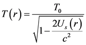(13)

where is the time rate of the clocks when. To first order, the predicted slowing of the GPS clocks is proportional to.

The 24 GPS satellites move round earth in six equally spaced 12 hours period orbits, with an orbital radius of 25,560 km and their orbital plane making 55 degrees with the earth’s equator. In the case of GPS satellites, having orbital plane nearly parallel to the earth-sun axis, the total slowing of the atomic clocks, during the 6 hours closer then earth from the sun, would achieve 24 ns, which would be recovered during the 6 hours farther from the sun. The GPS clocks normally are all collectively synchronized with the master clocks on ground to within 0.1 ns (time for light to travel 3 cm) and their stability during the 12 hours period of their orbits is better than 0.5 ns. Hence, the corresponding 12 hours sinusoidal variation in the time display of the GPS clocks, predicted by GR, due to the solar field, would be two decimal orders of magnitude larger than the stability and precision of these clocks during the period of the 12 hours and thus would immediately and easily be observed.

Clocks stationary within gravitational fields, confirm exactly the gravitational slowing according to Equation (13). As the gravitational potential is a scalar, a stationary or a moving clock should display exactly the same gravitational slowing and the rate of clocks at different distances from the sun should run at considerable different rates, according to Equation (13). However, the GPS clocks, moving with earth round the sun and, in their orbital motion, displacing their radial position from the sun by about, show no sign of the 12 hours periodic sinusoidal variation in the gravitational slowing [6] [7] . Obviously, the orbital motion of earth cannot cancel the solar gravitational potential. This absence of the solar gravitational slowing of the GPS clocks demonstrates that the gravitational clock slowing does not depend on the circular orbital distance from the sun, within the plane of the solar system. The in Equation (2) and in Equstion (13) cannot be the gravitational potential. It necessarily is the square of a velocity that is canceled by the orbital motion of earth. The only possible conclusion from this clear experimental observation is that the orbital motion of the GPS clocks with earth round the sun cancels the solar gravitational slowing. From the practical point of view this is fortunate, because otherwise the use of the GPS would be much more complicated. On the other hand however, this observation demonstrates that the gravitational potential is definitively not the cause of the gravitational time dilation. The absence of the solar gravitational slowing of the GPS clocks is the well-known noon-midnight problem that never has really been solved.

In order to understand the seriousness and the meaning of the absence of the gravitational slowing of the GPS clocks by the solar field, it is necessary to know the exact way the clocks count time. Clocks count time in terms of a time standard, which may be a classical or quantum oscillator. Actually, the best time standard, which is used in the atomic clocks, is the oscillation period of an electromagnetic (EM) cavity, tuned to the very precise frequency of the hyper- fine transition of gaseous alkali metal Cs atoms. The electromagnetic oscillations, within the tunable cavity and within the atomic cavities of the Cs atoms, are go-return round trips of the EM field, entirely analogous to that of the EM field of light in the light go-return round-trips between two mirrors. The difference is that the EM oscillations in the atomic structure involve the mass of the electrons of the atom. This is why atoms can emit radiation with wave lengths much longer than the size of the atoms. However, according to the previous Section II, the propagation velocity of EM fields (radiation) in the vacuum is fixed with respect to the local HQS. Hence, the frequency of light round-trips and of the EM oscillations within the Cs atoms are affected by motion of the laboratory with respect to the local HQS in exactly the same proportion. This is evident from several experimental observations, among which the best known are the Ives-Stilwell type experiments [27] . Consequently, measuring the velocity of light by the method of light go-return round-trips and a clock, necessarily gives always the same value, for any velocity of the laboratory with respect to the local HQS. This is the observational fact that underlies Einstein’s constancy of the velocity of light.

According to the previous Section II, the Higgs Quantum Space (HQS), ruling the motion of matter-energy, is locally the ultimate reference for rest and for motion for matter and light and effects of motion can only arise from motion with respect to the local HQS and cannot be caused by relative velocity. From this viewpoint, the absence of the gravitational slowing of the GPS clocks, moving with earth round the sun, by the solar field, demonstrates that earth is very closely stationary with respect to the local HQS. This obviously can make a sense only if the HQS is moving round the sun according to a velocity field, closely consistent with the orbital motion of earth. This conclusion emerges neatly from experimental observations and is not a guess. The correctness of this conclusion becomes really clear-cut, because a Keplerian velocity field, as will be shown in the coming Sections, accurately creates the gravitational dynamics on earth, in the solar system and in the galaxy and correctly generates all the observed effects of the gravitational fields on light and on clocks.

Time dilation is well known from the mean life-times of speeding Muons of cosmic radiation and from the red-shifts of the radiation emitted by speeding Hydrogen atoms [27] . In the STR, this time dilation is imputed to the relative velocity (). To first order the effect of this relative velocity is proportional to, where is the velocity of light. However, as earth is closely stationary with respect to the local moving HQS, the very high velocities of the Muons of cosmic radiation and of the Hydrogen atoms with respect to the earth-based laboratories in the Ives-Stilwell experiments is of course almost equally large velocity with respect to the local HQS. This will say that these observed time dilation effects can and must be due to their velocity with respect to the local HQS and not to relative velocity with respect to the laboratory.

The absence of gravitational slowing of the GPS clocks must be related with the absence of light anisotropy with respect to the orbiting earth, as is well known. The orbital motion of earth (30 km/sec) that suppresses the gravitational time dilation, due to the solar field, also suppresses the light anisotropy of 30 km/sec. On the other hand, the observed gravitational slowing of the atomic clocks, stationary on earth must be related with the small constant anisotropy of light of nearly 8 km with respect to the earth-based laboratories. In his most sensitive Michelson light anisotropy experiments, stop less day and night, Miller [28] has measured a nearly West-East light anisotropy of nearly 8 km/sec, constant the whole day and the whole year, exactly as predicted here. Please see details in Section III.2 below. This singles out the velocity with respect to the local HQS as the unified cause of time dilation and of light anisotropy and confirms the assertion, made in Section II, that velocity with respect to the local HQS is the origin of all effects of motion. In the absence of gravity, it is the ordinary velocity with respect to the local stationary HQS and, within gravitational fields; it is the implicit velocity with respect to the local moving HQS. Accordingly, time dilation has only one unique cause, the velocity with respect to the local HQS, as previously asserted.

The absence of the gravitational slowing of the solar field on the GPS clocks demonstrates that the gravitational slowing neither of stationary nor of moving clocks, within a gravitational field, is due to the gravitational potential. However, on the other hand, the observed gravitational slowing of the atomic clocks, stationary on earth, cannot be due to relative velocity, because these clocks are stationary with respect to the laboratory observer. These observations de- monstrate that neither the gravitational potential, nor the relative velocity can be the cause of time dilation. While the GPS clocks, moving with earth round the sun are stationary with respect to the local HQS that is moving with earth round the sun, the stationary clocks on earth are implicitly moving with respect to the local HQS that is moving round earth and through the earth-based laboratories. The present work will show that the HQS, ruling the motion of matter-energy, moving round the sun, round earth etc., is the quintessence of the gravitational fields and that this motion of the HQS accurately creates the observed gravitational dynamics and all effects of the gravitational fields on light and on clocks.

Obviously, earth cannot be kinematically privileged in detriment to all the other planets of the solar system and astronomical bodies in general throughout the universe. Earth is not the only planet that is com-moving with the local HQS in the velocity field round the sun. All the planets must be closely com-moving with the local HQS in the solar velocity field of the HQS. This will say that the HQS is moving round the sun according to a Keplerian velocity field, consistent with the planetary orbital motions. In order to be precise, let us define a system of non-rotating orthogonal (XYZ) coordinate axes, origin fixed to the gravita- tional center and let be the respective spherical coordinates and the unit vectors, pointing along the respective increasing spherical coordinates. The appropriate velocity field of the HQS that correctly creates the spherically symmetric gravitational field of the sun is a cylindrical velocity field, where the magnitude of the velocity is spherically symmetric:

(14)

Here is the Newtonian gravitational constant. For a given radial distance from the gravitational center the velocity along has the same value for all values of and. Figure 2 displays the velocity in the Keplerian velocity

field along one radial coordinate, which however is identical along any other direction. This spherical symmetry of the magnitude of the velocity, in the Keplerian velocity field of the HQS, assures the spherically symmetric solar gravitational field.

In the solar Keplerian velocity field of the HQS, the planets are all very closely stationary with respect to the local moving HQS, which directly predicts the null results of the Michelson light anisotropy experiments on earth, searching for light anisotropy, due to the orbital motion of earth. It also directly predicts the absence of the gravitational slowing, due to the solar field, of all clocks, moving with earth, or with any other planet, round the sun. In the Keplerian velocity field of the HQS round earth, consistent with the orbital motion of the Moon and creating the earth’s gravitational field, the velocity achieves nearly 8 km/sec on the earth-surface. However, the earth-globe rotates only very slowly (460 m/sec at the equator). This predicts the observed small clock slowing on earth and a small West-East light anisotropy of nearly 8 km/sec with respect to the earth-based laboratories, constant the whole day and the whole year. The time dilation and light anisotropy effects are very small, in the order of only 10⁻¹⁰ and thus extremely difficult to detect. Miller [28] and several other people, searching for light anisotropy with respect to the earth-based laboratory itself, have ob- served such small anisotropies (please see details at the end of the next Subsection III.2).

The Higgs field is a scalar field that is fundamentally different from the electromagnetic (EM) vector field. However, both the chargeless Higgs con- densate and the charged superconducting condensate (SCC) are quantum condensates, described by a complex order parameters, ruled by the principles of quantum mechanics. This is the reason of the close similarity in their phenomenologies. The meaning of Equation (14) is that a phase gradient () of the Higgs order parameter of the HQS is responsible for the velocity field of the HQS creating the Keplerian velocity field round the sun and round earth. In superconductors the EM vector potential, associated with the magnetic field, acts specifically on the charged SCC, creating a phase gradient in the superconducting order parameter and generating the velocity field of the SCC that screens and confines the magnetic field. An analogous vector potential, associated with the matter fields and acting specifically on the uncharged Higgs condensate, must induce a phase gradient in the Higgs order parameter, creating the velocity field Equation (14). Likewise the phase displacement of the SC order parameter is quantized along closed loops (Equation (12)), the phase change of the Higgs order parameter, along closed loops must satisfy an analogous quantization equation:

(15)

where is a constant depending on the mass within the closed integration loop, is an integration path and is the infinitesimal line element along the integration path.

The Higgs condensate (HC) is a strongly correlated quantum fluid, giving rise to considerable transient phase stiffness to the HC. Therefore, excitations in it cost large energies, because they necessarily must overcome the local strong phase correlation. However, once excited, the flow of the Higgs condensate along closed loops becomes lamellar, intrinsically quantized, very stable and persistent. Even if of the velocity field of the HQS is non-zero, the quantized flow lines in the velocity field Equation (14) is perfectly inviscid, however within limits. Only quantum fluids can exhibit this unique characte- ristic. They can so because their motion is governed by an order parameter, in which the flow along closed loops is quantized and diffuse motions are strongly suppressed by the BE correlation. The differential flow becomes viscous, rotational and dissipative only for large velocity differences (large velocity gradients) between neighboring quantized flow lines. The dependence of the Keplerian velocity field (Equation (14)), where is the spherical radial coordinate, is a universal characteristic of velocity fields of the HQS that is defined by the limit of the velocity gradient, on from which the flow becomes locally viscous, rotational and dissipative. Therefore, any perturbation in this dynamic equilibrium propagates out, in the form of gravitational waves, at the velocity of light, restoring the dependence.

In the large macroscopic Keplerian velocity fields (Equation (14)), generating the gravitational fields, the flow of the Higgs condensate along the coor- dinate is quantized, lamellar and inviscid and has very large quantum numbers in Equation (15). Despite, the flow in the form of quantized flow lines, encircling the whole gravitational source, is inviscid and free of local rotation. Only quantum fluids can exhibit this unique and fundamental characteristic. This property also is well-known in superconductivity, where the intensity of the quantized flow lines of the screening currents (velocity field of the superconducting condensate) falls exponentially with the distance from the core of the Abrikosov vortices (), where is the coherence length. Here, the vorticity of () is clearly non-zero. Despite this however, the velocity field is lamellar and inviscid. In the Keplerian velocity field of the HQS, an analog of the magnetic field, having a form similar to that of a magnetic dipole, too is present. However, the velocity field Equation (14) caries no electric charges. In Section IV, it will be seen that the fictitious Newtonian gravitational forces are the HQS analogs of the Lorentz forces in superconductivity. An analog of the electric field however is absent in the steady Keplerian velocity field. An analog of the electric field arises only if, which is the case in the collective velocity field of binary stars, generating gravitational waves (please see Section IV.3.11 for more details). However, in the case of star binaries, the oscillation periods are extremely long and the am- plitudes are low. The gravitational waves are strong enough to be detected on earth only in binary neutron-star merges or binary black-hole merges, as recently discovered [29] .

In view of the above comments, the origin of the gravitational dynamics must not be searched in terms of the usual methods of the classical fields. The gravitational dynamics involves no forces. It is ruled by inertial motion with respect to the local warping HQS in the Keplerian velocity field, creating the gravitational field. This inertial dynamics is governed by refraction of the de Broglie matter waves, due to the velocity gradient in the Keplerian velocity field, where the effects of the rotation round the gravitational center and the stretching/compression of the wavelength too must be considered. The problem is totally analogous to that of the well-known refraction in the propagation of sound waves in wind gradients or within whirl-wind [30] . Note that this gravitational mechanism is totally different from that of the central field of Newtonian gravitational forces and also is fundamentally different from that of the generalized inertial motions within the curved spacetime of GR.

In Section IV it will be seen that the Keplerian velocity field of the HQS, given by (Equation (14)), accurately gives rise to all the observed effects of the gravitational fields on matter, on light and on the clocks. The Keplerian velocity field round earth, in the sense of the Moon’s orbital motion, achieves 7.91 km/ sec on the earth’s surface and round the sun, in the sense of the planetary motions, it achieves 436 km/sec at the solar surface. A Keplerian velocity field of the HQS will be assumed to be circulating round each matter body throughout the universe, generating the respective gravitational field. A clock, stationary with respect to the ordinary space coordinates, within the Keplerian velocity field of a spherically symmetric mass, is implicitly moving at a velocity with respect to the local HQS. This velocity is implicit because it cannot be described with respect to the ordinary space. The gravitational slowing of such a clock, for longitudinal oscillation of the time standard, by which the clock counts time, is given by , where is the time rate for zero gravitational field. It is important to note that here is not the gravitational potential as in GR, however the square of the implicit velocity of the clock, the velocity with respect to the local HQS. In the final part of Section IV.1 it will be seen that the implicit kinetic energy, associated with this implicit velocity, is a centrifugal potential energy that corresponds to the usual gravitational potential. As this implicit velocity falls to zero for circular equatorial orbital motions, the velocity of light becomes isotropic and the gravitational slowing of clocks in such orbits is canceled, as observed for the GPS clocks.

3.2. Anisotropy of the Light Velocity

The interpretation of the Michelson light anisotropy experiments, searching for light anisotropy, due to the orbital and cosmic motion of earth depends funda- mentally on the view about the true motion of the earth-based laboratories. According to the conclusions in the previous Subsection III.1, earth is very closely stationary with respect to the local moving HQS, the ultimate reference for rest and for motions; in the solar Keplerian velocity field of the HQS and the solar system is com-moving (stationary) in the galactic velocity field. In the theory of relativity the orbital and cosmic motion of earth are seen as real, which has enforced the conclusion that the isotropy of light is intrinsic. This however, runs into conflict with the recently observed absence of the gravitational slowing of the GPS clocks, by the solar field, which demonstrates that earth is very closely stationary with respect to the local moving HQS, ruling the inertial motion of matter-energy, in the Keplerian velocity field creating the solar and the galactic gravitational field. The viewpoint of the theory of relativity also is inconsistent with the results of the one-way light anisotropy experiments, recently measured with the help of the tightly synchronized atomic clocks in orbit and to be described hereafter. In the Keplerian velocity field of the HQS, creating the earth’s gravitational field in the sense of the Moon’s orbital motion, and achieving nearly 8 km/sec on surface, the earth-based laboratories, on the very slowly rotating earth, are implicitly moving at nearly 8 km/sec toward the West.

In order to measure the one-way velocity of light, it is necessary having two tightly synchronized clocks, one at each end of the light one-way travel. According to the Special Theory of Relativity (STR), [2] [4] two clocks, resting at positions A and B in the inertial reference of the observer, can be synchronized by exchanging light signals between them. According to Einstein’s method, if a light signal is sent from A to B, at time of clock A, reflected back from B to A, at time of clock B, and arriving at A at time of clock A, then if, clock B is synchronized with clock A. This is exactly the condition for light isotropy within the inertial reference of the observer. According to the STR, the only restriction, for the synchronization to be possible, is that the clocks must be resting in the observer’s inertial reference. However, if clocks can be synchronized in such a simple way, why then has the one-way velocity of light not been currently measured? The problem is that within gravitational fields, where we live, the inertial references, located at different positions are mutually non-inertial so that, in practice, it is impossible to synchronize clocks at different positions within the earth’s field.

In the view of the present work, the velocity of light has a fixed value and is isotropic not with respect to all possible inertial references, however with respect to the local HQS, ruling the inertial motion of matter-energy. According to the previous Subsection III.1, the HQS is circulating round each astronomical body according to a Keplerian velocity field, consistently with the local main astro- nomical motions, thereby creating the respective gravitational fields. From this HQS dynamics viewpoint, Einstein’s synchronization method can succeed only if the two mutually resting clocks have no velocity component with respect to the local HQS along the straight line between the two clocks. Otherwise, the velocity of light will be anisotropic along the light path and synchronization will be impossible. In fact, the only essential requisite for clock synchronization to be possible is that the velocity of the electromagnetic signal (light) between the clocks, in the go and in the return journeys, be exactly the same at every point along the path, so that the times, in the go and in the return travels, are exactly the same.

The rate of the GPS clocks is preset before launch, so that their rate, when in orbit, equals that of identical clocks on ground. According to the present work, if the synchronization procedure of the orbiting clock with the master on ground is made when the satellite is nearly vertically above the ground station, then the velocity of the electromagnetic (EM) signal is perpendicular to the velocity of the HQS, in the Keplerian velocity field creating the earth’s gravitational field, along the whole signal path. As the velocity of the HQS is fixed at each point along the vertical signal path, synchronization of the GPS clocks with the master clock on ground, by Einstein’s method, can be very precise. Rapidly changing atmos- pheric conditions are the major source of errors.

Collective synchronization of the GPS clocks usually achieves 0.1 ns (time for light to travel 3 cm). With the help of such clocks, the one-way velocity of electromagnetic (EM) signals (light) between satellites has been precisely measured. Especially clear-cut measurement of the one-way velocity of EM signals (light) was achieved between the robotic twin satellites of the Gravity Recovery and Climate Experiment (GRACE) [31] . These twin satellites move in the same sense at nearly 8 km/sec along coplanar and practically identical circular polar orbits at about 500 km of altitude (vacuum), separated from each other by about 200 km and their positions being monitored by the GPS within 3 cm. Note that the Keplerian velocity field (Equation (14)), creating the earth’s gravitational field, has only a velocity component of 8 km/sec along the spherical coordinate and thus its effect on the light anisotropy along the polar orbit is irrelevant. Hence, the polar orbital velocity of the satellites is the relevant velocity for the one-way light anisotropy measurements between the satellites. The twin satellites of the GRACE project thus constitute a well-defined inertial reference and in order to measure micro-gravity effects, their atomic clocks continuously communicate with each other and need to be synchronized to better than 0.16 ns.

It has been observed that the signal transit time from the leading satellite to the rear satellite corresponds to a shortening by more than five meters (17 ns) over the 200 km. On the other hand, the signal transit time from the rear satellite to the leading satellite was lengthened by more than five meters (17 ns). These discrepancies are consistent with signal anisotropy, backward to the motion of the satellites, of nearly 8 km/sec, which is exactly the orbital velocity of the satellites. This anisotropy is two orders of magnitude larger than the experi- mental precision of the experiment and shows that the EM signal (light) has a well-defined and isotropic North-South velocity within the Geo-static non- rotating reference, the same with respect to which the satellites are moving at 8 km/sec.

This one-way anisotropy of light proves that a spatial medium (possibly the Higgs Quantum Space (HQS)) exists, propagating light at the characteristic constant velocity with respect to this medium and not with respect to Einstein’s inertial references. This result by it alone invalidates the fundamental assumption of the STR, according to which the velocity of light is intrinsically constant and isotropic with respect to all possible inertial references. The shortening and lengthening of the transit times by exactly the same value shows that the HQS, propagating light, is not moving along the North-South direction with respect to Earth (but may be moving along an West-East direction), exactly as given by the Keplerian velocity field of the HQS (Equation (14)), creating the gravitational field of earth. Therefore, the one-way anisotropy is due exclusively to the motion of the satellites. This experimental observation conclusively and definitively breaks the century old believes that the velocity of light is intrinsically constant and isotropic with respect to all possible inertial references. It in fact proves that the velocity of light is intrinsically constant and isotropic with respect to the local moving HQS.

The immediate consequence of this observed one-way anisotropy of light is that the current interpretation of the null results of the Michelson light anisotropy is false. This observation raises the absolute need of finding a new interpretation for all of the light anisotropy experiments, performed in the past century. Most of the Michelson light experiments aimed to measure the light anisotropy, due to the orbital and cosmic velocity of earth. Systematically, all these experiments obtained nominally null results. Now this must be interpreted as proving that earth as a whole has an irrelevant velocity with respect to the local moving HQS in the solar and in the galactic velocity fields etc. Obviously this can make a sense only if the HQS moves with earth round the sun and with the solar system round the galactic center etc. Hence, the observed isotropy of light with respect to earth simply reveals the true kinematical circumstance of earth with respect to the local HQS propagating light. This perfectly corr- oborates the previous conclusions that earth is a very specific preferred reference that is almost truly stationary with respect to the local moving HQS propagating light. This however is not the whole story. The null results of the light anisotropy experiments turn out to be exactly the signature of the true physical mechanism of gravity in action (please see Section IV).

The velocity field of the Higgs Quantum Space (HQS) round the sun, con- sistent with the Keplerian velocity of the planets, is a Keplerian velocity field of the HQS, creating the solar gravitational field and in which the orbiting planets are stationary with respect to the local moving HQS. However, a clock stationary with respect to the ordinary space, within this velocity field of the HQS, will be moving with respect to the local HQS at an implicit velocity. This velocity is implicit because it cannot be represented with respect to the ordinary space. This implicit velocity is the velocity that gives rise to the observed gravitational time dilation and light anisotropy, observed within gravitational fields.

The velocity diagram that must be considered in light anisotropy experiments within earth-based laboratories is displayed in Figure 3. If all the effects of motion are due to the velocity with respect to the local HQS, then, in Figure 3, the

rate of a clock depends on the effective velocity with respect to the local HQS, according to the equation:

(16)

where is the rate of the clock when it is stationary with respect to the local HQS (lower scale in Figure 3 at).

If the ordinary velocity of a clock increases from zero toward the right hand side () in Figure 3, its effective velocity with respect to the local HQS will first fall gradually from to zero, where the rate of the clock goes through a maximum when, showing proper time. This corresponds to the kinematical circumstance of the GPS clocks, in the solar field, moving with earth in the direct circular equatorial orbit round the sun. If the orbital velocity goes on increasing toward the effective velocity will grow up from zero and becoming increasingly more positive and the clock rate will fall gradually.

The experimental observation, described in Section III.1, demonstrate that earth is stationary with respect to the local moving HQS in the Keplerian velocity field of the sun and the solar system is stationary with respect to the local moving HQS in the galactic velocity field. Hence, the only remaining motion that can create light anisotropy and gravitational time dilation within the earth-based laboratories is the Keplerian velocity field of the HQS, in the sense of the Moon’s orbital motion and creating the gravitational field of earth itself. This velocity field achieves 7.91 km/sec from West to East on the earth’s surface and must create a light anisotropy of nearly 8 km/sec, due to the East-West implicit velocity of the earth-based laboratories. The anisotropy effect and spectral red-shifts of this low velocity is very small, in the order of only 10⁻¹⁰, direction fixed and value constant the whole day and the whole year. Such low anisotropy is very difficult to detect. Mössbauer experiments, [32] were sensitive enough to definitely measure the gravitational spectral red-shift on earth. Some genuine Michelson light anisotropy experiments, using highly sensitive Michelson interferometers, rotating within the earth-based laboratories, too were able to barely detect the very small anisotropy of light with respect to the earth-based laboratories. In his late and non-stop light anisotropy experiments, day and night, Miller [28] found small positive anisotropies of about 8 km/sec, nearly West-East, constant the whole day and the whole year, exactly as predicted above. Figure 4 displays the most complete anisotropy results obtained by Miller.

Light anisotropy experiments also have been made, using rather short maser

and laser cavities. Masers and lasers within these cavities are modulated into quantized modes, so that effects due to changes by less than one wavelength in the cavity cannot cause jumps between neighboring modes, which impedes such experiments to detect the very small anisotropies. From the present viewpoint, the light anisotropy experiments gave very low or null results, not because of the intrinsic isotropy of light, however because the velocity of earth with respect to the local moving HQS is much too low to give rise to easily detectable light anisotropies. The absence of the gravitational slowing of the GPS clocks, due to the solar field, the null results of the Michelson light anisotropy experiments and the one-way anisotropy of about 8 km/sec with respect to the GRACE satellites in a polar orbit are all the same and genuine signature of the HQS dynamic physical mechanism of gravity in action.

3.3. The Practical Significance of the Above Recent Experimental Observations

The experimental observations, described in the previous Sections III.1 and III.2 reveal key features that are crucial. They prove that the orbital motion of earth cancels the gravitational time dilation, due to the solar field, on clocks, moving with earth round the sun and hence cancels the spacetime curvature, introduced by Einstein, exactly to explain the orbital motion of the planets. Spacetime curvature thus cannot be the true origin of the observed gravitational dynamics. It obviously also cannot be the origin of the observed gravitational time dilation and of the gravitational slowing of the clocks, stationary within gravitational fields. These observations refute fundamental assumptions of the theory of relativity about the nature of space, about the meaning of motions and about the velocity of light. Visibly, the fact that earth is very nearly stationary with respect to the local moving HQS, ruling the motion of matter-energy, in the solar Keplerian velocity field and in the galactic velocity field etc., has mislead to the idea that the isotropy of light and the universality of the laws of physics are intrinsic and not circumstantial properties of nature.

In view of these observational facts, the present work associates together the central idea of the Higgs theory, according to which the HQS rules the inertial motion of matter-energy and the central idea of GR, according to which, gravitational effects are equivalent to inertial effects and replaces Einstein’s spacetime curvature by the Keplerian velocity field of the HQS Equation (14). Einstein's spacetime curvature explains the gravitational dynamics in terms of generalized inertial motions along the geodesic lines in the curved spacetime. However, the experimental observations, described in Section III.1, demonstrate that the orbital motion of earth cancels the gravitational slowing of the GPS clocks, due to the solar field and hence cancels the components of the Sch- warzschild metric tensor in Equation (2). This definitively turns GR unable to explain these orbital motions. These experimental observations also demonstrate that the Michelson light anisotropy experiments gave null results, not because of the intrinsic isotropy of light, however because earth is very closely stationary with respect to the local moving HQS, in the velocity fields of the HQS, creating the solar and the galactic gravitational fields etc. In reality, the Michelson light anisotropy experiments could well detect light anisotropy, due to the orbital and cosmic motion of earth. However, in its orbital and cosmic motion, earth simply is com-moving with the local HQS and hence it is stationary with respect to the local HQS in the velocity fields of the HQS, creating the solar and the galactic gravitational fields etc. With respect to the stationary earth, the velocity of light, excepting for the local effects of the earth’s field, is isotropic along all directions (North-South, East-West and Up-Down). However, in a reference, stationary in the gravitational field, like the earth-based laboratories, the velocity of light is slightly anisotropic along East-West, due the earth’s Kep- lerian velocity field along, where is the mass of earth. Along North-South or Up-Down directions, the velocity of light on earth is isotropic, however a bit lower than in free space, given by. In GR, the lower velocity along the radial coordinate is imputed to stretching of the radial distances (please see the radial term in Equation (2).

The Michelson light anisotropy experiments, searching for light anisotropy, due to the orbital and cosmic motion of earth, gave null results, because earth is almost stationary with respect to the local moving HQS and the anisotropy of light, due to these very slow motions, is in the order of only 10⁻¹³, much too small to be detected. On the other hand, the absence of the gravitational slowing of the GPS clocks by the solar field fully confirms these conclusions and thereby shows that earth effectively is almost stationary with respect to the local moving HQS. However, much more importantly: The Keplerian velocity field of the HQS, consistent with the local main astronomical motions, accurately generates the observed gravitational dynamics on earth, in the solar system, in the galaxies and throughout the universe (Section IV and V give the details). The null results of the light anisotropy experiments and the absence of the gravitational slowing of the GPS clocks by the solar field are both the genuine signature of the true physical mechanism of gravity in action that Einstein missed.

In the experimental tests of the theory of relativity, another crucial problem must be emphasized. All the experiments testing the predictions of the theory of relativity about time dilation, about relativistic mass and relativistic energy were made within the non-inertial earth-based laboratories, without any concern about the origin of this non-inertial character. Obviously this non-inertial character entails kinematical circumstances that were totally ignored in the interpretation of these experiments. Moreover, the very high velocity of the elementary particles or atoms and or light, used in these experiments, was many orders of magnitude larger than the implicit velocity of 8 km/sec of the earth based laboratories with respect to the local moving HQS in the Keplerian velocity field of the HQS creating the earth’s gravitational field. The velocities of most particles, used in these experimental tests, were comparable with the velocity of light. However, the clear-cut experimental observations, described in the above Sections III.1 and III.2, show that earth is very nearly stationary with respect to the local moving HQS, responsible for the light anisotropy, for the gravitational time dilation and for all the other so-called relativistic effects. If earth is almost stationary with respect to the local HQS, the effects that are usually imputed to the high relative velocities with respect to the earth-based laboratories can equally well and must be imputed to the high velocity with respect to the local HQS, with respect to which earth is almost truly stationary.

This means that, in Einstein’s expressions for time dilation, relativistic mass and relativistic energy, the relative velocity and the velocity of light must be replaced by the velocity of these particles and the fixed velocity of light with respect to local moving HQS. Although this entails radical conceptual changes, the predictions of the present HQS-dynamics approach, for experiments on earth are, within the usual experimental precision, identical to those predicted by the theory of relativity. The mistake committed in the interpretation of all these so-called relativistic experiments on earth is taking the earth-based laboratories as generic references, assuming that observers can arbitrarily stipulate the kinematical state of these earth-based laboratories. In fact, the recent experimental observations demonstrate that earth is very closely sta- tionary with respect to the local HQS, the ultimate reference for rest and for motions of matter-energy and thus earth, despite its orbital and cosmic motion, is a very specific preferred reference that is very nearly stationary with respect to the local HQS.

Only very recently have the measuring techniques achieved sensitivity enough to put in evidence the very small effects, in the order of 10⁻¹⁰, due to the implicit velocity of the earth-based laboratories of nearly (8 km/sec) with respect to the local moving HQS. With the vertiginous development of the scientific research technologies along the last hundred years, especially in fast electronics, com- puters and atomic clocks in orbit, the amount and quality of experimental data have enormously improved. These observations let clear that earth is very closely stationary with respect to the local HQS, in the Keplerian velocity field, creating the solar gravitational field. The effective velocity of the earth-globe with respect to the local HQS in the solar field is only a few hundred of meters per second. The effect of this small velocity is in the order of 10⁻¹³ and hence much too small to be detected even by the actual most sensitive and reliable experimental techniques. This explains the nominally null results of the light anisotropy experiments as well as the absence of the gravitational slowing of the GPS clocks by the solar field and most importantly, it straightforwardly and accurately generates the observed gravitational dynamics.

The disk shape of the solar system and of the galaxies as well as that of the natural satellite systems round the planets and the planetary rings all show that the orbits of the stable natural astronomical systems are closely concentrated within the equatorial plane of the respective Keplerian velocity field of the HQS. This minimizes their velocity with respect to the local HQS and turns their orbits very stable. The Moon is carried round earth at about 1 km/sec by the earth’s Keplerian velocity field of the HQS, the planets are carried round the sun by the solar Keplerian velocity field, the solar system is carried round the galactic center by the galactic velocity field of the HQS. All the astronomical bodies throughout the universe are nearly stationary with respect to the local moving HQS in the velocity fields creating the respective gravitational fields, which explains the universality of the laws of physics. This also will say that light is closely isotropic with respect to all these bodies and clocks in all these worlds display very nearly the universal proper time.

However, the universality of the laws of physics is not the same thing as covariance of the laws of physics in the theory of relativity. The Principle of Relativity is completely general and, according to it, no local experiment can detect the motion of earth, which leads to Einstein's general invariance or covariance of the laws of physics. However, the experimental observations, described in the above Sections III.1 and III.2, demonstrate that actually motions of the laboratory with respect to the local HQS can definitely be measured with the help of the tightly synchronized atomic clocks in orbit, as well as by light anisotropy experiments (Section III.2). They clearly show that the conventional light anisotropy experiments gave null results, not because of the intrinsic isotropy of light, however because earth is very nearly stationary with respect to the local moving HQS in the Keplerian velocity field of the sun, creating the solar gravitational field. The experiments simply were not sensitive enough to detect the very small effects of the very small velocity of earth with respect to the local HQS. The only experimental technique, having sensitivity enough, is the Mössbauer effect, measuring the spectral red-shift.

4. The Origin of the Gravitational Dynamics

The goal of this Section is clarifying the “modus operandi” of the HQS dynamics gravitational mechanism, generating the gravitational dynamics in the astro- nomical systems and on earth. According to the previous Section II, the Higgs mechanism is the HQS analog of the Meissner effect in superconductivity. In the presence of a magnetic field, a superconductor develops a screening velocity field of the superconducting condensate (quantized screening currents) that generate a Lorentz force field on the magnetic field, expelling it out from the super- conductor and or confining it into quantized magnetic fluxons or compressing it into macroscopic imprisoned magnetic flux bundles. This is the Meissner effect giving mass to the photons within superconductors. In the presence of matter fields, the HQS develops a Keplerian velocity field of the HQS (quantized screening flow) round the matter bodies that generates an inertial force field on the matter fields, thereby thrusting matter toward heavy bodies, confining matter into matter clumps and astronomical bodies. This is the Higgs me- chanism giving mass to the elementary particles and confining matter into macroscopic astronomical bodies. After Einstein’s equivalence of inertial and gravitational effects, the inertial force field, generated by the Keplerian velocity field of the HQS, is a gravitational force field.

4.1. Gravitational Dynamics in the Solar System

For clearness, consider again a system of non-rotating orthogonal (XYZ) Cartesian coordinate axes, origins fixed to the gravitational center and the Z axes pointing along the rotation axis of the solar system. This Z axis also is the rotation axis of the Keplerian velocity field of the HQS, creating the solar gravitational field. Let () be the usual spherical coordinates and () the unit vectors along the respective increasing spherical coordinates.

The experimental observations, described in Section III, demonstrate that the observed gravitational dynamics in the solar system is mostly motion of the HQS itself along the coordinate in the Keplerian velocity field of the HQS, created by the solar mass. The orbital motions of the planets are nearly circular and concentrate them closely within the equatorial plane of the solar Keplerian velocity field of the HQS. This minimizes their velocity with respect to the local HQS and is the reason why the solar system is disk shaped. The planets are simply carried round the sun by the moving HQS in the velocity field creating the solar gravitational field. The origin of this gravitational dynamics in the solar system thus is the solar Keplerian velocity field of the HQS. The very low velocity of the planets, of only hundreds of m/sec with respect to the local moving and warping HQS, is ruled by the principle of inertia, causing their orbits to be slightly elliptic. Effects of such low velocities on light and on clocks are in the order of 10⁻¹³ and thus much too small to be detected even by the actual most sensitive measuring techniques. Bodies in highly elliptic, non- equatorial and even retrograde orbits require relatively large velocities with respect to the local HQS. Such bodies with highly elliptic orbits end up captured by the central gravitational source, while those with very low velocity (with respect to the local HQS) avoid collisions and remain very stable in their circular equatorial orbits.

In the Keplerian velocity field, the HQS also contracts along certain directions and stretches along others, thereby changing the wavelengths of the particles along these directions and thus their velocity with respect to the local HQS, according to the de Broglie equation. However, along the and the directions, no such deformations of the HQS occur. Hence, if the effects of the Keplerian velocity field on the velocity of the de Broglie matter waves of the particles are expressed in terms of the effective rotation rates of the and the velocity components, the effects of the geometrical deformations are automatically taken into account and need not to be introduced explicitly.

Figure 5 is a very precise representation of the Keplerian velocity field of the HQS along, of the orbital velocity and the effective velocity of a small test body with respect to the local moving HQS. These velocities are represented at a large number of points along an elliptic equatorial orbit with eccentricity in the gravitational field of a central spherically symmetric source.

The purpose of this graphical representation is showing separately the be- havior of each of the three involved velocities, especially of the r and

components of. Intuitively it is clear that the Keplerian velocity field must rotate the and the r velocity components of in opposite senses. The problem is, knowing the exact rates. The rotation rates of the and the velocity components of can be read precisely enough in Figure 5. Specifically the rotation rate of the velocity component can be read at the top of the figure, while that of the velocity component can be read at the left hand side (please see ovals encircling the velocity diagrams). The horizontal dashed line, at each velocity diagram along the elliptic orbit, serves as a directional reference for estimating the rotations. Note that while the velocity component rotates clockwise, the velocity component rotates counter-clockwise and visibly with only one halve the rate of the component. The velocity component of, if it exists, does not rotate at all, because the Keplerian velocity field has no gradient in the plane and no component along the coordinate. The effective rotation rates (angular deflection rate) of the, and velocity components are:

(17a)

(17b)

(17c)

Note that the opposite rotation rates of the and the velocity components of characterizes not a trigonometric rotation of, however a hyperbolic rotation.

Free motion of matter bodies and the propagation of light within gravitational fields are governed by the set of Equation (17). If a matter body has an effective velocity with respect to the local HQS, the action of these rotation rates on the effective velocity components of the body makes the circular equatorial orbits elliptic. Depending of the magnitude of the velocity components, the refraction rates cause motion along parabolas, circles, ellipses or hyperbolas. Bodies having no orbital velocity () are extremely elliptic and correspond to the vertical fee-fall (the next Section IV.2 gives details).

4.2. Gravitational Dynamics on Earth

Matter immobilized with respect to the ordinary space non-rotating () axes within the gravitational field of a gravitational source, like earth, has considerably large implicit velocity (~8 km/sec on earth) along:

(18)

This velocity is implicit because it cannot be described with respect to the ordinary space. The implicit motion is ruled by the principle of inertia in the warping HQS of the Keplerian velocity field Equation (14) of. In terms of the rotation rate Equation (17b) and the implicit velocity Equation (18), the instantaneous rate at which vertical downward velocity (acceleration) of a small mass, with no orbital motion, is generated, is given by the vector product:

(19)

This is a spherically symmetric acceleration toward the gravitational center. For large gravitational sources, this gives rise to a relatively strong gravitational pull holding together the matter of the very slowly rotating source. This is the case of matter on earth and on large astronomical bodies in general throughout the universe. In fact all the gravitational sources rotate very slowly, much slower than the local HQS in the respective Keplerian velocity fields. This will say that the velocity of their matter has closely the value of the implicit velocity given by Equation (18).

Equation (19) is the usual expression for centrifugal accelerations in a rotating reference. In the Keplerian velocity field however the centrifugal acceleration points toward the gravitational center and the corresponding centrifugal forces are the fictitious Newtonian gravitational forces. This will say that a particle stationary with respect to the non-rotating (XYZ) axes must implicitly be moving along a circular path round an overhead axis.

The motion of particles, in fact takes place in terms of the de Broglie matter waves. The wave-fronts of a particle, stationary with respect to the ordinary space, (XYZ) axes and implicitly moving along, lie in the [] plain. As, in the Keplerian velocity field (Equation (14)), the velocity of the HQS, along and through the [] plain, increases for decreasing, these wave fronts see a velocity distribution of the HQS that locally corresponds to a rotation of the HQS and thus of the local Inertial Reference (IR) round an overhead axis. The direction of the overhead axis is along and will be shown to be located at a position. Moreover, in the Keplerian velocity field, the local IR is a different one at each point of space. A particle, stationary with respect to the () axes, will implicitly be moving within the local rotating IR, along an opposite implicit circular path round the overhead rotation axis of the local IR under an upward centripetal acceleration. In order to the particle move so, a real upward centripetal force (mg) must be acting on it. In the absence of such an upward centripetal force, the free particle will follow an inertial path within the local IR, implicitly moving along an instantaneous straight line within each local rotating IR that it happens to pass. As the local IR is rotating round the overhead axis, the implicit velocity vector of the particle will rotate together with the local IR at this same rate. This rotation of the implicit velocity (Equation (17b)) develops a real vertical downward velocity component that an observer in the implicitly upward accelerated (non-inertial) earth-based laboratory interprets as gravitational acceleration of the free-fall.

The HQS is of course not rotating round an overhead axis, however is circulating round the gravitational center. The rotation of the local-IR round the overhead axis takes place only in the view of the wave fronts of the particle that lie in the [] plane. In fact, the local rotation of the HQS in the velocity field, given by Equation (14), is intermediate between the rigid-body rotation and the irrotational potential flow. Therefore, wave fronts of a particle, having an ordinary velocity component along the coordinate, lying in the [] plane; do not see the rotation round the overhead axis. They see the opposite rotation of the HQS round the gravitational center, given by Equation (17a). This rotation is reminiscent of waves propagating in a medium in rigid body like rotation. Very similar refraction effects occur for sound waves propagating within wind gradients or within whirlwind [30] . Finally, the wave fronts of a particle, having a velocity component only along the polar () coordinate, that lie in the [] plane, are not refracted at all, because the Keplerian velocity field (Equation (14)) has no velocity component normal to the [] plane.

Note that, within the gravitational source, the velocity of the HQS in the velocity field goes on increasing inward the spherical body according to. However the velocity gradient gradually decreases and falls to zero at the center of the gravitational source, thereby zeroing the gravitational acceleration.

Equation (19) is sufficiently precise only for free-fall along short distances. In order to describe the free-fall of a test mass m along large distances in the field of a large mass M, it is necessary to use the elementary homogeneous linear differential equation:

(20)

where the left-hand side is the acceleration, is the distance from the gravitational center and, is the column matrix of the (ordinary) and the (implicit) velocity components of the free-falling body:

(21)

In the right-hand side of Equation (20), is the hyperbolic infinitesimal rotation matrix, defined in terms of the rotation rates, given in Equation (17):

(22)

where and accounts for the asymmetric distribution of velocity and kinetic energies between and as well as for the explicit time dependence of the velocity field due to motions of the source with respect to the center of mass, under the field of. For, and for,

The acceleration, in the left-hand side of Equation (20) has two components. An ordinary acceleration component along the ordinary coordinate and an implicit acceleration component along. The ordinary acceleration along is produced by acting on the implicit velocity component of the particle along, which is the usual gravitational acceleration. On the other hand, the implicit acceleration along is produced by, acting on the ordinary velocity component. This last accele- ration increases the implicit velocity along.

Solving the differential Equation (20), generates the velocity components in the formal way. Inserting the matrices and into equation (20), dividing both sides by, multiplying by and integrating the left hand side from to, develops into:

(23)

which can be written in the exponential form as:

(24)

Expanding the exponential in series and adding up the terms of the series from to results in:

(25)

where can be computed by integrating the infinitesimal angular rotations swept from to:

(26)

Inversion of the final term of Equation (26) results in the hyperbolic cosines and sine as a function of:

(27a)

(27b)

Using this result and noting that, Equation (25) becomes:

(28)

For free fall of m in the field of, on from and initial rest, where and, the final solution of Equation (20) is:

(29a)

(29b)

Equation (29a) is just the well known expression for the observed vertical free-fall on from rest at and Equation (29b) is just the implicit velocity as a function of the radial position with conservation of the angular momentum about the gravitational center. The vertical velocity is just times larger than the implicit velocity along, which accomplishes the Virial theorem. Note that in this treatment of the gravitational dynamics in no place is there invoked a gravitational force or anything similar. This clearly shows that gravity is not a fundamental force, however an emergent phenomenon created by HQS-dynamics. Moreover, it is clear that the velocity of all bodies throughout the universe with respect to the local HQS is very small, so that the, so called, relativistic effects are totally irrelevant. In the case of a matter body having zero velocity with respect to the local HQS, the effects of refraction (Equation (17)) vanish and the body simply accompanies the local motion of the HQS round the gravitational source, which is closely the kinematical circumstance of earth and all the planets in the solar system.

The implicit velocity component of a mass, falling in the field of, given by Equation (29b), cannot be described with respect to the ordinary space

coordinates. It is an imaginary quantity and the corre-

sponding implicit kinetic energy is negative:

(30)

This negative energy is an implicit kinetic energy term, which in reality is a centrifugal potential energy that must be interpreted as the gravitational po- tential energy. However, potential energy necessarily involves at least two bodies. In the case, too is implicitly moving in the field of at an implicit velocity and the corresponding centrifugal potential energy is:

(31)

Adding up Equations (30) and (31), which are identical in value, gives the usual expression for the total potential energy:

(32)

The corresponding total ordinary kinetic energy is the sum of the kinetic energies of and of, due to their ordinary velocity along the radial coordinate, toward the center of mass, given by Equation (29a). However, as (), practically the whole kinetic energy is stored by and:

(33)

This equation shows that the kinetic energy of the free falling mass, on from rest, is equal to the variation in the potential energy. Considering the solutions Equation (29), conservation of the total mechanical energy of a free-falling body in the gravitational field of may be expressed in terms of the hyperbolic sine and cosine functions as:

(34)

where the term is related with the potential energy and the term is related with the kinetic energy as a function of time. This total mechanical energy is an invariant, as long as no external force acts on the system.

4.3. Symmetry of the HQS-Dynamics Gravitational Mechanism with Orbital Motions

Consider vertical free-fall experiments with small particles on the surface near to the equator of a spherical planet of radius, rotating at an angular velocity round the same axis as the Keplerian velocity field HQS, generating the gravitational field. The effective velocity of a particle, initially resting near to the surface of the rotating planet, with respect to the local HQS will be:

(35)

where is the ordinary velocity, due to the planet’s rotation that depends on the latitude via and the upper and lower signs are respectively for direct and retrograde rotation of the planet with respect to that of the local HQS.

For rotation of the planet in the same sense as the HQS in the Keplerian velocity field, the clockwise trigonometric rotation rate of of the particle, due to the planets rotation, adds up to that of the HQS, given by Equation (17b). However, for retrograde rotation it subtracts, so that the effective rotation rate of the effective velocity vector of the small free particle on the rotating planet’s surface is:

(36)

where the same convention for the upper and the lower signs as in Equation (35) is used.

Considering the effective velocity (Equation (35) and the effective angular velocity (Equation (36), the effective gravitational acceleration on the planet’s surface is:

(37)

The first term in the right hand side of Equation (37) describes the acceleration toward the gravitational center in the static situation [see Equation (19)], while the second term is an outward centrifugal term. This shows that the effective gravitational acceleration on the rotating planet’s surface is perfectly symmetric for direct or retrograde rotation of the planet, that is, for direct of retrograde orbital motion of the particle. Note that, at the equator, is maximum when and, independently from, when. The effective gravitational acceleration at the equator even becomes upward for.

For strictly circular polar orbits with radius, has velocity components along as well as along. The velocity along is:

(38)

Along theta the velocity is:

(39)

While generates the gravitational acceleration, see Equation (19), the velocity component is not affected directly by the HQS- dynamics, because the velocity field Equation (14) has no velocity component along theta. Hence, the effective gravitational acceleration for polar orbits is:

(40)

where the first term in the right hand side is the acceleration toward the gravitational center [see Equation (19)], that plays the role of a centripetal acceleration in the polar orbit, while the second term is the corresponding usual upward centrifugal effect.

An analytical solution of Equation (20) for more general orbital motions is not at all easy. However, the results, expressed by Equations (37) and (40), reveal a feature that circumvents this difficulty. From these equations, it is clear that the effect of the HQS-dynamics is completely independent from the effects of the ordinary dynamics. The effects of the implicit and the ordinary motions are orthogonal. Effectively, the implicit velocity of a particle has no meaning from the viewpoint of the ordinary space and the ordinary motion has no meaning from the viewpoint of the local implicitly rotating references, because to each point in space there corresponds to a different implicitly rotating inertial re- ference.

While the Keplerian velocity field of the HQS (Equation (14) simulates a central field of fictitious Newtonian gravitational forces, the orbital motions generate the centrifugal effects, exactly as conceived in Newtonian gravity. This shows that treating the general motions within the spherically symmetric velocity field Equation (14) as motions in a hypothetical extended inertial reference, under a hypothetical central field of fictitious gravitational forces generating the gravitational acceleration and the free fall. This explains why the Newtonian gravitational theory, although based in the fictitious gravitational forces, works so well.

In conclusion, the Keplerian velocity field (Equation (14)) of the HQS, ruling the inertial motion of matter and the propagation of light, consistently with the local main astronomical motions, simply carries the planets along circular equatorial orbits round the sun. There is no need of a central force field and no need of a curved spacetime. Each planet is very closely stationary with respect to the local moving HQS, which straightforwardly explains the nominally null result of the light anisotropy experiments as well as the absence of the gra- vitational slowing of the GPS clocks. The very slow motion of the planets, with respect to the local warping HQS in the solar Keplerian velocity field, is ruled by the principle of inertia, according to Equation (17), which causes the weak orbital ellipticity. The gravitational effects, generated by the Keplerian velocity field of the HQS Equation (14), is orthogonal to the effects created by the ordinary motions.

4.4. The Effects of the HQS-Dynamics Gravitational Fields on Light and on Clocks

The previous Subsection III has shown that the Keplerian velocity field of the HQS (Equation (14)) correctly creates the observed gravitational dynamics on earth and in the solar system. The purpose now is showing that this Keplerian velocity field also correctly predicts all the effects of the gravitational fields on the propagation of light and on the rate of clocks, there including all the new effects, recently discovered with the help of the tightly synchronized atomic clocks is orbit.

4.4.1. The One-Way Velocity of EM Signals between the GRACE Satellites

The most precise measurements of the one-way velocity of EM signals (light) were obtained with the help of atomic clocks, tightly synchronized to within 0.1 ns (time for light to move 3 cm), between the robotic twin satellites of the GRACE project. These clocks were moving in the same polar orbit, at 500 km of altitude and nearly 200 km from each other (please see details in the above Section III.2). The exchange of EM signals in both senses, between these satellites showed a clear anisotropy of the signal velocity of nearly 8 km/sec backward to the motion of the satellites [31] . This anisotropy is exactly equal to the orbital velocity of these satellites and as the velocity field Equation (14) has no component along the polar coordinate, this observation is perfectly con- sistent with the predictions of the present HQS-dynamics.

4.4.2. The Michelson Light Anisotropy Experiments

The large majority of the Michelson experiments searched for light anisotropy, due to the orbital and cosmic motion of earth. They all found closely null results, which corroborates the assertion of the present work that earth is very closely stationary with respect to the local HQS, in the Keplerian velocity field (Equation (14)), creating the solar gravitational field. The next Section V will show that the solar system is stationary with respect to the moving HQS in the galactic velocity field. The absence of the solar gravitational time dilation on the GPS clocks fully corroborates this same fact. In the view of the present work, the only motion, that causes relevant anisotropy of light and clock slowing, within the earth-based laboratories, is the local velocity field of the HQS (Equation (14)) round earth itself in the sense of the Moon’s orbital motion and creating the earth's gravitational field. This velocity reaches 7.91 km/sec on surface and the corresponding light anisotropy is constant in value and direction the whole day and the whole year. Setting in Equation (16) of Section III.2, gives the gravitational time dilation on earth. Moreover, Figure 3 displays the velocity diagram for anisotropy experiments within the earth field (please see the point where. The most precise Michelson experiments, searching for light anisotropy with respect to the earth-based laboratories, using Michelson inter- ferometers of the highest sensitivity and rotating within the earth-based laboratories, found anisotropies of nearly 8 km/sec, approximately constant the whole day and the whole year, [28] exactly as predicted here with base in the HQS-dynamics gravitational mechanism. Please see the anisotropy results by Miller, plotted in Figure 4 in Section III.2. With base in the known astronomical motions, the aether theories expected light anisotropies with respect to earth not smaller than 230 km/sec. Miller’s small anisotropy results simply could not comply with these expectations and therefore were ignored by the scientific community, alleging possible systematic errors. Michelson, Morley as well as Miller, instead of recognizing that the null light anisotropy demonstrate that earth is stationary in the medium ruling the motion of matter-energy and generating the gravitational dynamics, tried to explain the smallness of the anisotropy results in terms of aether entrainment by matter. In the scenario of the HQS, this hypothesis is nonsense, because the HQS, ruling the motion of matter-energy, is an unbelievably powerful spatial medium that carries earth and the other planets round the sun and rules the whole dynamics of the universe. Matter-energy is not more than foam of weak perturbations in this medium. Other light anisotropy experiments with maser and laser cavities too gave null results. However, visibly such cavities are intrinsically unable to measure small light anisotropies like those, due to the earth's Keplerian velocity field (more details in the end of Section III.2).

4.4.3. Gravitational Time Dilation and Gravitational Spectral Red Shifts

The gravitational time dilation or gravitational slowing of clocks and the gravitational spectral red-shifts on earth are now well confirmed experimentally [32] [33] [34] . Within the Keplerian velocity field of the HQS (Equation (14)), creating the earth’s gravitational field, the gravitational slowing of the clocks is given by:

(41)

where, the effective velocity with respect to the local moving HQS is closely equal to the implicit velocity Equation (18) for zero orbital velocity and is the fixed velocity of light with respect to the local moving HQS. This effective velocity arises from the Keplerian velocity of the HQS, creating the earth’s gravitational field, through the laboratories on the very slowly rotating earth- globe. To first approximation, the gravitational slowing of clocks, stationary on earth and light anisotropy experiments is proportional to, where is the mass of earth. Within the earth-based laboratories this effect is only about 10⁻¹⁰ and thus very difficult to detect. Mössbauer spectral red-shift ex- periments on earth [32] have shown effects of exactly this value. The atomic clocks on earth also closely showed gravitational time dilation of this value [34] . The depends on the orbital velocity and is zero for direct circular equatorial orbits round earth or round the sun as observed for the GPS clocks. GR predicts gravitational time dilation of the same value, however based in a completely different physics, in which the gravitational time dilation is due to the gravitational potential. However, the gravitational slowing of the GPS clocks by the solar field, predicted by GR, is not observed (please see Section III.1 for details). This shows that the gravitational potential is not the cause of the gravitational time dilation. The nuclear, atomic and molecular energy levels certainly adjust them to these gravitational time dilation effects.

4.4.4. The Excess Time Delay of Radar Signals in the Solar System

According to GR, massive astronomical bodies cause curvature of the spacetime geometry in their neighborhood. Spacetime curvature symmetrically lengthens the go-return path of electromagnetic (EM) radiation passing closely by these bodies, giving rise to an excess time delay. Shapiro [35] has measured this excess time delay within the solar system by time keeping the transit time of radar signals for complete go-return round-trips from earth to Venus and back to earth, during about two years. The excess time delays showed a cusp-like peak near to the superior conjunction of Venus (please see Figure 9 below), in conformity with the predictions of GR.

The present work treats the excess time delay of the radar signal round-trips between earth and Venus as an effect of propagation in the moving HQS, creating the solar field and ruling the velocity of the radar signals. From this viewpoint, the excess time delay is not caused by the increased geometrical distance, however to the effective velocity of the radar signals within the Keplerian velocity field of the HQS round the sun. During the direct signal journey, the solar velocity field is favorable, increasing the effective velocity. However, during the retrograde journey the velocity field is unfavorable, decreasing the effective velocity. According to well known physics, in such round-trips the loss of time in the retrograde journey is larger than the gain in the prograde journey, so that an effective excess time delay results in a complete go-return round-trip. The problem is totally analogous to that of light round- trips within a laboratory, moving with respect to the local HQS. The calculation of the excess time delay within the solar Keplerian velocity field however is a little bit complicated because the velocity of the signal depends on the position. The excess time delay thus must be calculated by integration.

In the present work, the excess time delay of the radar signal round-trips was calculated numerically and separately for the go and for the return travel along straight line paths from earth to Venus and back to earth, as displayed in Figure 6, using the effective velocity. This calculation was repeated for a series of paths, having the minimum distances from the center of the sun (impact parameters): R = 0, 2, 4, 8, 25, 50 and 100 million km, before and after superior conjunction (please see results in Table 1 and plotted in Figure 7). The excess time delays were numerically calculated, dividing the straight line paths in a large number of segments (about 420 segments, shorter segments near to the sun), computing the excess time-loss and time-gain, separately for the transverse and for the longitudinal components of the solar Keplerian velocity field along the signal paths for each segment and finally adding up (integrating) the contributions along the whole path. More than 99% of the excess-time-delay or gain comes from the longitudinal component of the solar velocity field along the path. In the calculation, the different Earth-Venus distances, due to their orbital positions as well as the different signal path (slightly different R), due to the motion of earth during each signal round-trip were taken into account.

The results show that although the travel times for individual Earth-Venus and Venus-Earth journeys is considerably asymmetric (please see Figure 7, the

effective excess time delay for the full earth-Venus-earth round-trips, fourth column in Table 1 and displayed in Figure 8, practically coincide with the excess time delays measured by Shapiro, [35] and displayed in Figure 9. In the HQS-dynamics, this effective excess time delay is a simple and genuine physical effect, due to the effective signal velocity within the solar Keplerian velocity field of the HQS and not to the increase of the geometrical distance due to the spacetime curvature of GR. The fact that the Keplerian velocity field of the HQS

round the sun correctly produces the effective excess time delay (Shapiro effect) fully corroborates the present HQS-dynamics gravitational mechanism.

Other precise measurements of the excess time delay (Shapiro Effect) of signals passing close to the sun have been made with the help of Mars landed transponders during the Mariner 6 and Mariner 7 missions as well as other spacecrafts (Cassini). However, all these experiments measured the effective excess time delay for complete go-return signal round-trips and hence could in no way detect the anisotropy in the velocity of the signals in the go and the return journeys, shown in Table 1 and displayed in Figure 7.

4.4.5. The Gravitational Light Lensing Effect

The gravitational light lensing effect was first predicted by Einstein [3] [4] . According to the present work, consider two light beams, from two distant stars and propagating directly toward the sun, initially along parallel paths, as shown in Figure 10. First, in the region where the velocity of light has almost only radial components, the wave vectors are refracted according to Equation (17a) by a total angle, thereby the light beams gaining a small velocity com- ponent along, which exactly compensates the drag by the velocity field along. This reduces its radial velocity component to. Near to the sun, where the solar velocity field achieves 436 km/sec and is mostly parallel (left) and anti-parallel (right) to the beams, refraction by Equation (17b) is dominant and the wave vectors are refracted oppositely by a total angle. Finally, after going away in the opposite side, the wave vectors are refracted again according to Equation (17a) by nearly an

angle. However, near to the sun, the solar velocity field is favorable to the prograde ray (left side of Figure 10) so that it spends less time near to the sun and hence is deflected by a smaller angle. To the retrograde ray however (right) the solar velocity field is unfavorable and hence it spends a longer time near to the sun and refracts by a larger angle. This differentiated refraction by by Equation (17b) causes a convergence of the rays that is responsible for the gravitational light lensing effect.

The angle can be calculated simply by multiplying the refraction rate Equation (17b) times the excess (or shortage) of time delays listed in Table 1. On the solar surface and the refraction rate, given by Equation (17b), is. Interpolating the value of in Table 1 for light passing by the surface of the sun, we find the excess time delay at the retrograde side of closely and a shortage at the prograde side of. The product gives, which is very closely the observed deflection angle, causing the convergence of light passing close to solar surface.

4.4.6. Non-Simultaneous Arrival of a Pulsar Signal along the Orbital Motion of Earth

The aberration of star light is an old and well known feature in astronomical observations from earth. Usually it is explained in terms of the orbital velocity of earth. However, according to the present work, this aberration contains an additional unperceived feature that arises from the refraction rate of light, propagating toward the sun, according to Equation (17a) by an angle so that, where is the velocity of the HQS in the solar Keplerian velocity field. Figure 11 shows qualitatively the effect of this refraction rate. This refraction rate creates a velocity component of the light signal toward and thereby reduces the radial velocity component to. Corre- spondingly it slants the wave fronts by and angle. In midnight telescopic observations from earth, the telescope must be inclined by an angle, pointing along the direction indicated in Figure 11 by, along which the wave fronts are perpendicular to the path of light within the telescope and the velocity of light has exactly the usual value within the telescope.

Astronomical observations with the help of interferometric methods can improve the images by orders of magnitude. This is achieved with the help of computers by coherently superposing the digital images (signals) received by separated telescopes or radio-astronomy antennas, taking into account the dis- tances of the antennas from the observational field. The fundamental requisite for this method to work is that the superposed signals received in the different observatories be synchronous. This is achieved with the help of atomic clocks, closely synchronized with the help of the GPS clocks. However, on testing the synchrony of the clocks along the Very Long Base Line Interferometry set-ups, by the arrival of the millisecond pulsar signals, there was a surprise. The arrival

of the pulsar signals to the antennas of terrestrial antenna array equidistant from the pulsar, along directions transverse to the earth’s orbital motion, was synchronous, as expected from the theory of relativity. However, to antenna arrays of equidistant antenna arrays from the pulsar along the orbital motion of earth the arrival was out of synchrony, up to 4.2 microseconds for antennas at diametrically opposite sides of the earth-globe. This observation frontally con- tradicts the expectations from the theory of relativity and has raised a controversial about the synchronization of the GPS clocks [6] [7] .

From the viewpoint of the HQS-dynamics, the wave fronts of signals coming from a distant pulsar toward the sun, sketched in Figure 12, are slanted, due to refraction according to Equation (17a). The slanting angle at the point of observation is such that, which on earth is equal to the usual aberration angle of star light (please see Figure 12). Because of this slanting of

the wave fronts, the non-synchronous arrival of the pulsar signal to the eq- uidistant earth-based observatories, along the orbital motion of earth, is real. Hence, there is no reason for suspicions about the synchronization of the GPS clocks.

4.4.7. The Perihelion Precession

The perihelion precession is one of the most important predictions of Einstein’s GR [3] [4] . From the viewpoint of the present work, an analogous differentiated refraction rate of the and velocity components of of an orbiting body as for light in the preceding Section IV.3.5, must be responsible for the peri- helion precession of elliptical orbits. At the aphelion the direction of the effective velocity, with respect to the local HQS, is opposite (retrograde) to the velocity field of the HQS as well as to the orbital motion. This increases the time of permanence in this region of the orbit. As the refraction rate is a characteristic of the position, the velocity vector of the particle refracts during a longer time. However, at the perihelion is parallel to the velocity field (prograde), which displaces it more rapidly (than the HQS) in the velocity field, so that it has not enough time to recover the tangential direction. It recovers it only somewhat beyond the ideal perihelion point. In this way the perihelion advances a little bit in the prograde sense in each orbital round-trip.

4.4.8. Absence of Gravitational Slowing of the GPS Clocks by the Solar Field

In the view of the present HQS-dynamics gravitational mechanism, the slowing of clocks is caused by velocity with respect to the local HQS and not by relative velocity. Hence, clocks, stationary with respect to the local moving HQS, run not slow. They show proper time. The velocity of the GPS clocks, moving with earth round the sun, with respect to the local HQS is given by:

(42)

Hence, the GPS clocks are stationary with respect to the local moving HQS in the solar Keplerian velocity field. Therefore, these clocks cannot show gravita- tional slowing, due to the solar field, as effectively observed for the GPS clocks [6] [7] . All clocks orbiting in circular equatorial orbits round an astronomical body, which normally orbits itself in a regular circular equatorial orbit round a larger body (star or galaxy), are stationary with respect to the local HQS. Such clocks, if identical, run all synchronous with respect to each other and all show closely the same proper time throughout the universe.

4.4.9. Effects of the Velocity Field of the HQS on Clocks Moving in Non-Equatorial Circular Orbits

Clocks moving round earth along circular polar orbits have, besides the implicit velocity along, given by Equation (18), the velocity of the same value along the polar orbit. Hence, their effective velocity with respect to the local HQS is and their slowness is two times larger than that of identical clocks resting at the same altitude. Moreover, the velocity with respect to the HQS of clocks in retrograde circular equatorial orbits is and their time dilation is four times larger than that of an identical clock resting in the gravitational field at the same altitude. In particular, the GPS satellites move at of altitude, along circular orbits inclined 55 degrees with respect to the earth’s equator and hence have a considerable average velocity with respect to the local HQS in the Keplerian velocity field creating the earth’s gravitational field. The GPS clocks have velocity components, given by along and along, where and is the angle of the orbital velocity with respect to the equator or parallels. The effective velocity is and the estimated average velocity of the GPS satellites with respect to the local HQS over the entire orbit is. Considering in addition the velocity of 0.22 km/sec of the Cs atoms in the atomic clocks along the orbital motion, this makes 3.30 km/sec with respect to the local HQS. Analogously, for the earth based stations we find 7.20 km/sec with respect to the local HQS. Using these values (), we find that the rate of the GPS clocks must be slowed by before launch in order to these clocks to run approxi- mately synchronous with identical clocks resting on ground. This is approxi- mately the value by which NASA slows the rate of the GPS clocks before launch.

4.4.10. The Astronomical Motions Closely Track the Motion of the HQS throughout the Universe

The null results of the light anisotropy experiments, due to the orbital and cosmic motion of earth and more emphatically, the absence of the gravitational time dilation on the GPS clocks, due to the solar gravitational field, proves that the planet earth is stationary with respect to the local HQS that rules the propagation of light. From the HQS-dynamics point of view, the planetary orbits lie all closely within the equatorial plane of the solar Keplerian velocity field of the HQS and the orbit of the solar system lies closely within the galactic disk, which is the equatorial plane of the galactic velocity field of the HQS. Hence, the planets as well as the solar system are com-moving with the HQS. All these bodies minimize their velocity with respect to the local HQS. This minimization visibly is the result of the wavelength stretching, due to the expansion of the universe and the velocity averaging down of random opposite motions during agglomeration into large matter bodies. The expansion of the universe must have stretched the wavelengths of the particles analogously as it has stretched that of the photons, as is well known from the cosmic microwave background radiation. This certainly has reduced the velocity and the momentum of the particles, according to de Broglie’s equation, with respect to the local HQS, as well as the kinetic energy of the particles.

4.4.11. Gravitational Waves

Einstein was the first to predict the occurrence of gravitational waves. In the view of the present work, binary star systems necessarily generate oscillations (per orbit) in their collective velocity field of the HQS. They generate oscillations as a function of time in the value of, as well as in the magnitude of the itself, where is the HQS analog of the EM vector potential (please see Section III.1). The oscillation in is the HQS analog of an oscillating magnetic field and the is the HQS analog of the electric field. These oscillations propagate out as gravitational waves at the velocity of light. However, the gravitational waves, generated by star binaries, have low amplitudes and very long oscillation periods and hence their energy is much too low to be detected from earth. However, neutron star binaries or black-hole binaries are very compact systems that achieve, during the merges, orbital velocities comparable with the velocity of light, generating oscillations of enormous amplitude and an increasing frequency that may achieve hundreds of Hz. The problem is that black-hole merges, besides unpredictable and extremely rare in the universe, last for only a few seconds. Due to the enormous distances, they reach us red-shifted and strongly attenuated (fortune for us, misfortune for the researchers). This makes the detection of the gravitational waves extremely difficult. Recently, however after many decades of intense efforts, the LIGO Scientific Collaboration and the Virgo Collaboration research groups have achieved the feat. They have detected the characteristic profile of gravitational waves, due to a very distant binary black-hole merger [29] .

5. The Observed Rotation of the Galaxies without the Need of Dark Matter

While more than 99% of the mass of the solar system is concentrated in the central sun, more than 99% of the mass of galaxies is orbiting in the form of stars round the galactic center. Our Milky Way Galaxy is an old barred spiral galaxy, having a central bulge of about 10⁴ light years across, where it harbors a super- massive black hole. The bulge is surrounded by a thin disk-shaped swarm of hundreds of billions of stars, orbiting along closely circular orbits and extending out to about 4.5 × 10⁴ light years.

Many published works [36] [37] [38] display orbital velocity profiles, obtained by spectroscopy measuring methods, for the stars in galaxies as a function of the distance from the galactic center. In many galaxies, the orbital velocity increases with the distance from the galactic center. Figure 13 displays an observed velocity profile of our Milky Way Galaxy, [38] together with a typical Keplerian rotation curve. From the viewpoint of the current theories, the rotation rate of the galactic disks are much too fast to be hold together by gravity, produced by their content of visible matter.

The discrepancies between the theoretical predictions and the observations, instead of having raised suspicions about the current theories of space and gravitation, have lead to distrusts on the observational means of the astronomers. It is alleged that a huge halo of invisible dark matter is present, causing the non-Keplerian rotation of the galaxies. The amount of dark matter however is estimated to be about 5 times larger than that of visible matter. This dark matter is extremely exotic. It does not scatter, absorb and emit electromagnetic

radiation, but interacts with ordinary matter only by gravity. However, why then is dark matter not concentrated within stars and galaxies? The non-Keplerian galactic rotation is actually among the most challenging impasses in the current theories about the nature of space and gravitation.

Another way to address the problem of the peculiar galactic rotation rate, is by the gravitational potential. The gravitational potential has been com- puted [39] as a function of the distance from the galactic center for our Milky Way galaxy as well as for other galaxies. Systematically all these computed gravitational potentials are inconsistent with the observed orbital motions of the stars in the galactic disk.

The gravitational potential can of course be obtained empirically using the Virial theorem of classical physics and the circular orbital velocity profile of the stars like that in Figure 13. For central gravitational force fields, the gravitational potential has a very simple relation with the circular orbital velocity:

(43)

The galactic gravitational potential curve, obtained in this way, is shown in Figure 14 and is to be seen as the true observed potential. Please notice that within the galactic disk, the gravitational potential is closely leveled, which means that the force field toward the galactic center is almost zero (). Despite this however, the stars are moving along circular orbits round the galactic center. From the usual mechanics point of view, this breaks fundamental principles of physics and seems absurd. From the view of the HQS dynamics gravitational mechanism however this is perfectly reasonable, because it is the HQS itself that is so moving and carrying the stars around. Likewise the solar field carries the planets round the sun, the galactic velocity field carries the stars round the galactic center. There is no need of a central force field. However, why does the solar velocity field fall as, while the velocity field of the galaxy does not

fall and even increases with in many galaxies? The next Sections V.1 and V.2 give the response.

5.1. Binary Stars Unveil the Key Feature That Is the Origin of the Non-Keplerian Rotation of the Galaxies

The crucial question to be answered is: Why do the orbital velocities of the planets decrease with distance from the sun according to (Equation (14)), while the orbital velocities of the stars in the galactic disk do not fall and in many galaxies even increases with? This is the observational fact that the current theories of gravitation cannot explain, without postulating a huge amount of dark matter. The goal here is showing that the gravitational theory, based in the present HQS-dynamics, predicts this non-Keplerian galactic gravitational dy- namics even with details without the need of dark matter (see also Ref. [40] ).

In the view of the current gravitational theories, effects of motion of the gravitational sources on their gravitational fields become important only for very high velocities, close to the velocity of light. Here, it will be shown that, motion of a gravitational source can create important effects on the Keplerian velocity field of the HQS, creating the gravitational field, even at relatively low velocities.

In order to highlight the relevance of the effects of the orbital motion of the gravitational sources on their Keplerian velocity fields, let us begin with the simple case of a binary star system. Assume that the rotation axes of the Keplerian velocity fields of the individual stars are perfectly aligned and that the sources are moving along a circular equatorial orbit round the center of mass (CM) in their collective velocity field and that their individual Keplerian velocity fields are rotating in the same sense as the orbital motion. Otherwise it can be shown that they would not form a bound system. These stars will be com-moving with the local HQS along circular orbits in the equatorial plane of the collective velocity field of the HQS, creating the gravitational field of the binary. Otherwise their orbits cannot be circular.

The gravitational dynamics of the binary system can be well described by Newtonian mechanics. Balance of the mutual Newtonian gravitational forces and of the opposite centripetal force on each star leads to the observed orbital velocity of each star round the CM:

(44)

where is the distance between the two stars and is a positively defined length. Consider now a small test particle moving round an equal, however isolated and static mass in a circular equatorial orbit having the radius. The orbital velocity of this test particle is considerably larger:

(45)

Equation (44) and Equation (45) are correct and simply describe the obser- vations. However, while in Equation (45), the gravitational source remains stationary at the CM and the orbiting test particle is com-moving with the local HQS in Keplerian velocity field (Equation (14)) of the source, in the case of Equation (44) the sources are both com-moving with the HQS in the collective velocity field of the HQS, otherwise their orbits would in no way be circular. However, why are these velocities so different?

In the view of the present work, the difference between Equations (44) and (45) unveils a key feature that plays a fundamental role in the non-Keplerian gravitational dynamics of galaxies. This difference discloses the effect of the relatively slow orbital motion of the individual gravitational sources on their Keplerian velocity fields of the HQS, creating their respective gravitational fields. This however will not say that, from the viewpoint of a local observer on or on, the gravitational fields on the individual stars lose their spherical symmetry. In fact, locally the Keplerian velocity fields retain their spherical symmetry, excepting only for small tides.

The only possible reason for the reduced velocity of the HQS in the binary velocity field, at the position of the individual stars of the binary, is their orbital velocity round the center of mass (CM). From the viewpoint of a stationary observer in the non-rotating (XY) axes, the orbital velocity of the sources, given by Equation (44), subtracts from the individual spherically symmetric velocity fields Equation (14) toward the inner side, however adds up to it toward the outer side, as depicted in Figure 15.

In order to fully put in evidence the effects of motion of the gravitational sources on their velocity fields, consider now in addition a small test particle moving in the collective velocity field of the binary, along a direct circular orbit within the orbital plane of the binary. The orbital velocity of such a test particle is of course given by, where is the distance from

the CM of the binary. This orbiting particle is of course com-moving with the local HQS. For large, the velocity of the HQS in the collective velocity field round the binary is:

(46)

In order to reconcile the addition of the velocity fields of the two sources outside the binary with the velocity in the collective velocity field (Equation (46)), the same orbital velocity that reduces the velocity fields toward the inner side, must enhance them outward the binary orbit. At distances much larger than, the addition of the velocity fields of and must reproduce the value, given by Equation (46). Note however that, because the velocity fields Equation (14) of the individual sources depends on the square-root of the source mass, the addition of the velocity fields, due to the different sources must satisfy the sum rule:

(47)

Taking into account this sum rule, the collective velocity field, for large, takes the form:

(48)

Solving for of the mass along the axis and for gives:

(49)

A totally similar result is valid to the left hand side of, where.

With this result, the external collective velocity field of the binary, for large and or large, gives:

(50)

which reproduces the result of Equation (46) for large.

These results show that effectively the same orbital velocity that reduces the velocity fields of the individual sources by a factor toward the inner side of the binary (Figure 15), enhances their velocity fields by a factor toward the outer side. The reason clearly is the orbital velocity of the sources in the static (XY) plane. Note however that, outside the binary, the effect of the orbital motion on the collective velocity field is not seen from large distances. At large distances, the gravitational effect is the same as in the static case (zero orbital velocity).

In conclusion, while toward the inner side, the orbital velocity, subtracts from the spherically symmetric velocity fields (Equation (14)), according to Equation (47):

(51)

outward the binary, the orbital velocity adds up to the spherically symmetric velocity fields (Equation (14)):

(52)

The results expressed by Equations (51) and (52) and plotted in Figure 15 are a unique feature of the present HQS-dynamic gravitational mechanism. None of the current theories of gravitation can give rise to these features. In Figure 15, going along the positive X axis, on from the CM, there is an upward velocity step, from to, created by.

(53)

Note that here Equation (47) needs not to be considered, because the velocities refer to the same mass. Going toward the left hand side, there is an analogous downward velocity step at the position of. These velocity steps are a fundamental feature in the building up of the velocity field of the HQS, ruling the non-Keplerian galactic gravitational dynamics.

The obvious conclusion from the above analysis is that the Keplerian velocity fields of the individual stars in the galactic disk act in the sense of opposing the Keplerian decrease of the galactic velocity field. In some galaxies this effect is strong enough to invert the velocity gradient so that the velocity, within the disk effectively increases with. Beyond the border of the galactic disk, where the mass density falls strongly, the galactic velocity field of course tends to the Keplerian dependence.

In-between the orbiting stars of the binary, the velocity fields of the HQS of and, reduced by the orbital velocity, are opposite to each other and also opposite to the external velocity field (please see Figure 15). Along the X axis, the addition of these internal velocity fields, according to Equation (47), gives:

(54)

Near to the effective internal velocity is upward and close to it is downward. At the origin (CM) there is a stagnation point, where the effective velocity falls to zero.

5.2. The Observed Non-Keplerian Rotation of the Galaxies without the Need of Dark Matter

The previous Sub-section V.1 makes a quantitative analysis of the gravitational dynamics of a binary star system, from the viewpoint of the new theory of the HQS-dynamics gravitational mechanism. Putting an increasing number of stars, moving in the same sense along the same circular orbit round the CM, the oppositely rotating internal and the directly rotating external velocity fields of the HQS become increasingly larger and smoother. Figure 16 displays a sketch of the collective velocity field, created by a system of eight equal stars, the in- dividual velocity fields of which rotate round parallel axes in the same sense as the orbital motion. The figure shows that the velocity in the internal collective velocity field is much smaller and opposite to the external velocity field. A stagnation point exists at the center as well as between each pair of stars. The stars simply move with the local HQS round the CM.

In order to the stars in a galaxy create a coherent collective velocity field, it is necessary that the velocity fields of the individual stars be fairly well polarized, their velocity fields rotating in the same sense about parallel axes. In the solar system the planets and their satellites rotate and move along orbits practically all in the same sense along nearly circular equatorial orbits within the plane of the solar system. This demonstrates that the Keplerian velocity fields, creating the gravitational fields of all these bodies are highly polarized and rotate in the same sense round axes nearly parallel to the axis of the solar system. In the galactic disk, the stars too are orbiting all in the same sense along circular equatorial orbits round the galactic center. The rotation axis of our solar system is known to make about 63 degrees with respect to the rotation axis of the Milky-Way galaxy. This deviation may be related with the spiraled structure of the galaxy. Presently, there are no data to define the orientation of the stellar Keplerian velocity fields of the HQS in the Milky-Way galaxy. It however seems reasonable to assume that the stellar velocity fields are fairly well polarized, creating the galactic gravitational dynamics.

Precise computation of the velocity field of a galaxy, containing hundreds of

billions of stars, obviously requires formidable computational means. Here only a qualitative estimate is possible, which however convincingly shows that the HQS-dynamics gravitational mechanism consistently and naturally leads to the observed non-Keplerian rotation of the galaxies, even with details.

In order to extend the model, consider now multiple concentric and coplanar circular orbit loops with larger and larger radii and each loop containing a very large number of stars, moving in the same sense round the CM. Figure 17 is a representation of the velocity profile of the velocity field of the HQS as well as of the estimated effective velocity of the stars (blue line) through four successive loops in an intermediate region of for a case in which the number of stars in each loop is constant with the distance from the galactic center, which means nearly equal velocity steps (Equation (53)) in each loop.

According to Equation (53), in which is proportional to the total mass of the star loop, each star loop acts in the sense of opposing the characteristic Keplerian decrease in the velocity field, creating locally an upward velocity step. If the star density as a function of is constant, the velocity of the HQS in the collective velocity field as well as the orbital velocity of the stars

within the galactic disk necessarily increase with. If the star density decreases moderately, the velocity may become constant with and if the star density falls steeply, the velocity field regains the Keplerian dependence.

From the viewpoint of the current gravitational theories, the stars in the galactic disk too attenuate the (inward) slope of the negative gravitational po- tential within the galactic disk. However, in these theories the profile of the gravitational potential depends only on the position of the gravitational sources and not on their orbital velocity. Therefore, they cannot reproduce the obser- vations.

The star loop model is only a qualitative description. It however can con- vincingly explain the observed gravitational dynamics of galaxies and even predict incredible details, without the need of dark matter. For instance, if the mass density increases very steeply with, the velocity in the velocity field increases even more steeply. This is not a guess. The observed velocity profile of our Milky Way galaxy in Figure 13 shows a profound depression and possibly even retrograde rotation close to the galactic center, where the star density becomes low. This depression at the origin is a general feature, present in most observed galactic velocity profiles. If the mass density is very low in an extensive region near to the center, the star loop model predicts the formation of a central region, where the rotation is in the retrograde sense. In many galaxies, such retrograde rotation of the inner part of the galaxy is effectively observed. NGC 7331 is an example of a galaxy in which the bulge rotates in a sense opposite to that of the external disk [41] . However, many other examples exist. Beyond the galactic border, where the star density begins to fall steeply to zero, the velocity field recovers the Keplerian dependence on from its value at the galactic border (please see Figure 13).

The planets in the solar system too constitute a disk round the sun, however of irregular and a very low mass density, less than 1% of the matter of the solar system. They however too must attenuate a little bit the solar Keplerian velocity field until the border of the solar system, where it regains the Keplerian de- pendence. This has the consequence of increasing a little bit the solar gra- vitational acceleration on going beyond the border of the solar system. This may explain the Pioneer anomaly, which is a very small but well-defined (anomalous) increase in the gravitational acceleration of the Pioneer 10 and Pioneer 11 spacecrafts toward the sun, observed as they moved beyond the border of the solar system in two opposite directions [42] [43] . To now this anomalous effect never has got an explanation.

The null results of the Michelson experiments, searching for light anisotropy due to the orbital and cosmic motion of earth, demonstrate that the solar system, despite its orbital velocity of about 230 km/sec round the galactic center, is very closely stationary with respect to the local moving HQS ruling the propagation of light. However, our solar system can of course not be a privileged exception. All the stars within the galactic disk must equally be closely com-moving with the HQS. Otherwise their orbits would not be circular. This confirms that the equator of the galactic velocity field of the HQS, creating the galactic gravi- tational field, coincides with the galactic disk. The stars are of course not constrained to move along these circular orbits by gravitational forces and these circular motions also cannot be explained in terms of spacetime curvature of GR, because the circular equatorial orbital motions cancel the gravitational time dilation and hence the spacetime curvature, as demonstrated by the absence of the gravitational slowing of the GPS clocks by the solar field (please see Section III.1). The stars are simply carried along circular equatorial orbits by the galactic velocity field of the HQS, analogously as the planets are carried round the sun by the solar Keplerian velocity field. These stars are stationary with respect to the local HQS, analogously as earth and the other planets are resting with respect to the local HQS in the solar velocity field. This explains the observed isotropy of light with respect to earth in spite of the orbital motion round the sun and in spite of the orbital motion of the solar system round the center of the Milky Way galaxy. Moreover, identical clocks com-moving with earth and with the solar system or with any other star in the galactic disk, are stationary with respect to the local HQS and run all naturally synchronous, showing all the same universal proper time.

The fact that, within the galactic disk, the velocity of the HQS is constant as a function of the distance from the galactic center, implies a nearly zero velocity gradient as well as a zero potential gradient and thus a nearly zero refraction rate of light passing within the galactic disk. However, beyond the border of the galactic disk, where the velocity field recovers the Keplerian dependence, the refraction rate may be strong. This effect is analogous to the light lensing effect of light passing near to the sun (please see Section IV.3.5.) The refraction rate in the galactic border however is much weaker than that near to the sun. However, while the light lensing effect by the sun is produced in about 13.5 milliseconds of excess time delay, the excess time delay of light, traversing the border of the galaxies is in the order of many years and hence it may result in a considerably large angular deflection, forming round heavy galaxies circular silhouettes of refracted light coming from light sources in the back of these galaxies or even large irregular silhouettes of refracted light round heavy galactic clusters, as observed in several compact galactic clusters.

6. Dark Energy, Vacuum Energy and the Cosmological Constant

Astrophysical observations prove that the expansion of the universe is accele- rating. Evidence of this accelerated expansion has been found independently from measurements of supernovae of type Ia [20] [21] as well as from microwave background radiation [22] . With base in the Friedman Equations (4) and (5) (please see Introduction), cosmologists have imputed the origin of this accelerated expansion to a dark energy, usually viewed as a constant vacuum energy density, obeying the equation of state, where is a spatially homogeneous negative pressure and. To present date however, the nature of dark energy is a mystery.

Although a mystery, the presence of dark energy is actually an indubitable observational fact. The consensus among the cosmologists is that dark energy is not ordinary mass-energy, but is energy of space itself, energy of the vacuum, which distributes it very homogeneously throughout the universe. It also is consensus that dark energy interacts with ordinary matter-energy only by gravity. However, these conclusions, although plausible from the viewpoint of the observations, are made without indicating the physical background, able to give rise to these features. The present work will show that all these features arise naturally and appropriately within the scenario of the global Higgs Quantum Space (HQS) dynamics (see also Ref. [44] ).

From the viewpoint of particle physics, the cosmological constant in the Friedman-Lemaitre-Robertson-Walker universe, Equations (3), (4) and (5), plays the role of a vacuum energy density, accelerating the expansion of the universe. In this scenario, the empty spacetime (vacuum) usually is modeled in terms of the four-dimensional energy-momentum tensor of a perfect fluid, with a positive vacuum energy density and an isotropic negative pressure:

(55)

where is the fluid four-velocity.

In the empty space (vacuum), the ordinary mass-energy density is zero and the fluid is static. In this condition, the stress-energy tensor can be equated to the vacuum energy density. The current theories estimate the vacuum energy density from the perspective of the elementary particle physics, com- puting the zero-point energy of an infinite number of independent oscillators. They normally include zero point oscillations of the various scalar fields with spontaneously broken symmetry, like that of the broken chiral symmetry of the strong interaction (QCD), of the broken electroweak symmetry etc. From the perspective of the particles physics, the density of the vacuum energy does not decrease with the expansion of the universe and hence the expansion of the universe creates energy, which leads to the negative pressure. Altogether, these contributions lead to the theoretically estimated vacuum energy density of, which is 120 decimal orders of magnitude larger than the observed value, obtained from observations of supernovae of type Ia [20] [21] as well as from microwave background radiation [22] . The observed energy density is only. These facts show that there is obviously something absolutely wrong in the assumptions of particle physics, underlying this pro- cedure.

In the scenario of the Higgs theory, the vacuum is filled up with the scalar Higgs field with spontaneously broken symmetry, described by an order parameter with a non-zero vacuum expectation value and a total associated condensation energy, given by:

(56)

where is a uniform constant energy density of the Higgs condensate, corresponding to the number of bosons per unit of volume. The coefficients n and m are constants, where (please see Section II for the details). The potential in Equation (56) has a minimum for, which is the depths of the potential well.

The Higgs Quantum Space (HQS) is responsible for giving mass to the elementary particles by the Higgs mechanism and thus rules the inertial motion of matter-energy and necessarily is their locally ultimate reference for rest and for motion. The Higgs potential well in Equation (56) is generic to each point of space and its depths is the same throughout the universe, which can explain the flatness and the horizon problem of cosmology.

According to the Glashow-Weinberg-Salam electroweak model, the energy gap between the unbroken and the broken electroweak symmetry is in the order of 200 Gev, which is the depths of the potential well Equation (56). However, the Higgs condensation is a second order phase transition (no latent heat) and liberates this amount of energy gradually along its route toward zero tem- perature. In the BE condensation of the usual superfluids and superconducting condensates, the energy, liberated by the condensation, is removed by efficient cryogenics. However, in the case of the HQS, there is no external world to absorb the huge amount of energy and entropy. There is no exchange of energy or of work with an external world. The expansion of the universe thus necessarily is adiabatic and the total energy in it must be conserved. The only way to the universe reducing its energy density is by increase of volume. Expansion stretches the wave lengths of the particles and of radiation, reducing their energy and hence the temperature of the universe. As far as observations show, the universe has no boundary and no barriers and thus the expansion is free and necessarily accelerated (potential energy converts into kinetic energy). The process is analogous to the expansion of warm and humid air in the formation of clouds, however in the absence of an external pressure.

The energy of the Higgs condensate (HC) within the energy well Equation (56) is not usual mass-energy, however energy of the Higgs condensate itself, energy of the vacuum. This energy depends on the volumetric density, the boson density. If or, the energy of the HC is not minimum. However, if, it can lower its energy by accele- rated and adiabatic volumetric expansion. Observations show that actually the expansion of the universe is accelerating. This indicates that. However, if, the HC can lower its energy by contracting.

In the HQS scenario, modeling the vacuum energy from the perspective of particle physics in terms of the zero point energy of independent oscillators certainly is inadequate, because the HQS can in no way be seen as a perfect fluid of independent particles, nor can its vacuum energy be estimated in terms of the zero point energy of independent oscillators. In perfect fluids, the particles are uncorrelated and have their symmetry preserved. They cannot develop collective and cooperative effects, because the hypothetical particles and oscillators are uncorrelated and all independent. Therefore, perfect fluids cannot confine fields. For instance, it is well known that a perfect electrical conductor has no Meissner effect and a perfect fluid cannot give rise to a Higgs mechanism.

In contrast superfluids, superconductors and the HQS, have broken symmetry and are dominated by collective effects. These quantum fluids are strongly correlated systems, in which the BE correlation strongly suppresses local phase fluctuations and hence local motions. Quantum condensates con- stitute an integrated entity, where the particles are quantum mechanically identical and indistinguishable. In the quantum condensates, the principle of uncertainty is singular, which means that, for all practical instances, the uncer- tainty in position of the particles tends to infinity and the momentum is well defined, the uncertainty in time is infinite and the energy is well defined. The motions of such condensates are ruled by an order parameter, in which all excitations are intrinsically quantized and persistent. In a quantum condensate it is impossible to interact with only a part of the condensate. Any interaction always affects the order parameter and thus all the particles. This enables the quantum fluid to develop strong collective and cooperative effects, confining perturbing fields, minimizing their effects and providing them with inertial mass. Quantum condensates are like an army troupe, where any attack always is an attack against the whole group and will have the response of the whole troupe. Therefore, a quantum condensate behaves wholly like one unique oscillator.

The potential well of the Higgs condensate in Figure 1 is represented in terms of the amplitudes of the real and imaginary components of the order parameter. The form of this potential well is generic to each point of space and its deepness necessarily is the same throughout the universe. It is analogous to the electro- static potential well of an infinite homogeneous superconducting metal (Nb) piece at very low temperature, where the BE correlation well extends over the whole metal piece and has the same depth throughout the whole piece. In the case of the Higgs, the potential well has the size of the universe. This will say that only zero-point oscillations with infinitely long wavelengths are possible. This lets clear that the energy contribution of the zero-point oscillations (vacuum fluctuations) in the HQS are irrelevant. In fact the observed effects of the vacuum fluctuations (Casimir effect and the Lamb shift) in Quantum Electro- dynamics are of electromagnetic nature. The electromagnetic field has its symmetry preserved and is not a quantum condensate.

In the scenario of the HQS, the deepness of the Higgs potential well in the Glashow-Weinberg-Salam electroweak model is fixed. However, actually the matter universe, together with its vacuum (Higgs condensate), lies deeply within the Higgs potential well Equation (56), though still not at the bottom. The situation is analogous to that of the superconducting condensate (SCC) in an infinite superconducting metal piece at very low temperature, under an applied magnetic field, where too the thermal phase fluctuations and of the phase perturbations by the magnetic field hold the SCC back from its true minimum of energy. In the case of the HC, the perturbing fields that hold back the advance of the HC toward the minimum of energy are the matter fields, due to the presence of the ordinary matter-energy. Therefore, the effective energy density of the HC is not minimum ().

To parameterize the actual vacuum energy density (effective energy density of the HC) in terms of the volume is difficult, because of the initial inflation period. The size of the universe in the epoch of electroweak symmetry breaking is not well known. The temperature of the universe however is a better parameter. Along the expansion of the universe, its temperature fell from the initial 10¹⁵ K, at the beginning of the electroweak symmetry breaking, to the actual low temperature. The cosmic-microwave-background radiation leads to 2.7 K. How- ever, because of the high temperatures within and in the neighborhood of the stars and galaxies, the average temperature of the universe certainly is somewhat higher than 2.7 K. Perhaps 100 K is a good guess. From this viewpoint, the energy density of the universe fell from the initial 200 GeV to the actual, which corresponds to nearly 10⁻¹⁰ ergs/cm³, or equivalently to about 10⁻²⁹ g/cm³. However, although the mass density is very low), it distributes it uniformly over the whole universe, so that the integrated energy is 14 times larger than that of the whole visible matter-energy in the universe.

There is a fundamental difference between the present approach and the ap- proach of particle physics. In the present approach the total energy of the universe is conserved. The expansion of the universe only lowers the energy density. It does not create new energy as it does from the perspective of particle physics.

The actual small residual vacuum energy density consists of two parts: The condensation energy that still has not decayed because temperature is not really zero (bare cosmological constant) and the major part that is hold back by the local phase perturbations of the Higgs order parameter due to the presence of the ordinary matter-energy in the universe. The present estimate, while giving vacuum energy density values in agreement with the observations, also solves the intriguing coincidence problem of cosmology. Why are actually the values of the vacuum energy and of the visible ordinary matter-energy so closely equal? According to the present work, the phase perturbation of the Higgs order parameter by the ordinary (visible) matter-energy is responsible for the HQS dynamics (gravitational dynamics) throughout the universe and thus for the major part of the residual vacuum energy. It hence is no surprise that the actual vacuum energy and the ordinary visible matter energy are so closely equal.

On the other hand, the only relationship of the HQS, with ordinary mass- energy, is giving mass and ruling the inertial motion of the elementary particles. This will say that the only way of the HQS-dynamics (vacuum energy) to affect the motion of ordinary matter-energy is by inertial effects, which after Einstein's equivalence of gravitational and inertial effects are gravitational effects.

In conclusion, dark energy is not ordinary mass-energy, but energy of the HQS itself, of the vacuum itself. The total vacuum energy is closely similar to the total visible matter-energy because it is the visible matter-energy that holds back the Higgs condensate from the minimum of energy. As the HQS is a quantum fluid, pervading all of space, this energy necessarily distributes it very homogene- ously throughout the universe. Moreover, the HQS, ruling the inertial motion of matter-energy, interacts with ordinary matter-energy only by inertial effects that are equivalent to gravitational effects. This shows that the HQS-dynamics naturally meets all the characteristic properties of dark energy that are con- sensual among the cosmologists. It however entails a fundamental additional feature: The accelerated expansion of the universe necessarily is accelerated expansion of the HQS itself.

Experimental Evidence That the Accelerated Expansion of the Universe Is Accelerated Expansion of the HQS Itself

The recent experimental observations, [6] [7] achieved with the help of the tightly synchronized atomic clocks in orbit and described in Section III, demonstrate that the HQS, ruling the inertial motion of matter-energy, is circulating round earth, round the sun and round every astronomical body throughout the universe, according to Keplerian velocity fields, consistent with the local main astronomical motions. The Keplerian velocity field of the HQS is the quintessence of the gravitational fields. In the velocity field of the sun, earth is very closely stationary with respect to the local moving HQS and, in the velocity field creating the gravitational dynamics of the Milky Way galaxy, the solar system is stationary with respect to the local moving HQS. The observed absence of the gravitational slowing of the GPS clocks by the solar field and the isotropy of light with respect to earth perfectly corroborate this view. In fact these observations are the authentic signature of the physical mechanism of gravity in action.

However, while the local HQS-dynamics round the sun and round the galactic center properly explains the isotropy of light with respect to earth, it cannot explain why the recession between the galaxies causes no light anisotropy. An appropriate explanation of the accelerated expansion of the universe can of course not run into conflict with the null results of the Michelson light anisotropy experiments. The fact that the velocity of light is isotropic with respect to earth, despite its motion in the solar system and the motion of the solar system in the Milky-Way galaxy and also in spite of the relative motion and recession between the galaxies, demonstrates that the accelerated expansion of the universe too lets earth stationary with respect to the local moving HQS. Despite the accelerated expansion of the universe, our Milky-Way galaxy remains stationary with respect to the local HQS. It certainly would not be reasonable to assume that our galaxy is in a privileged kinematic circumstance with respect to the HQS in detriment to all the remainder galaxies in the universe. All the galaxies must equally be closely stationary with respect to the local HQS. These facts inexorably lead to the conclusion that the HQS, ruling the inertial motion of matter and the propagating light, besides moving according to velocity fields, consistent with the local main astronomical motions and thereby creating the observed gravitational dynamics, also is expanding consistently with the recession of the galaxies. This will say that the Hubble spectral red-shift of light from distant galaxies and the red-shift of the cosmic microwave back- ground radiation, are not usual Doppler shifts, but are due to a time-rate of stretching of the wavelength, due to the adiabatic expansion of the HQS, their medium of propagation. It is easy to show that this stretching, as a function of time, causes exactly the same red-shift as the usual Doppler shift, due to conventional recession. It also stretches the wavelength of the particles, thereby reducing their velocity and kinetic energy with respect to the local HQS, according to the de Broglie equation (). The velocity of oppositely moving matter particles is moreover averaged down during the gravitational agglomeration into astronomical bodies. This largely explains why the velocity of all the major astronomical bodies with respect to the local HQS is actually so small throughout the universe.

In summary, the HQS, ruling the inertial motion of matter and the pro- pagation of light, is circulating round earth, round the sun and round the galactic center, consistently with the local main astronomical motions, thereby creating the observed gravitational dynamics. In the local HQS-dynamics round the sun and round the galactic center, earth is very closely stationary with respect to the local HQS, so that the orbital motion of earth and the motion of the solar system within the galaxy cause no light anisotropy with respect to earth. Moreover, the accelerated expansion of the matter universe is consistent with the accelerated expansion of the HQS itself, in this way too letting earth, the solar system and the Milky-Way galaxy and all the other galaxies stationary with respect to the local HQS. This concomitant expansion ultimately explains the observed isotropy of light with respect to earth. It also predicts the universality of the laws of physics and that all clocks, moving together with the natural astronomical bodies run nearly synchronous and show closely the universal proper time throughout the universe.

7. Conclusions

The present work investigates the consequences of the recent experimental observations, achieved with the help of the tightly synchronized atomic clocks in orbit round earth, within the scenario of the Higgs Quantum Space (HQS). These experimental observations, demonstrate that the HQS, ruling the motion of matter-energy, is not static, but is moving round the sun, consistently with the planetary orbital motions and certainly round each astronomical body through- out the universe, according to Keplerian velocity fields, consistent with the local main astronomical motions. The Keplerian velocity field of the HQS is the quintessence of the gravitational fields. It directly and naturally explains the orbital motions of the planets round the sun and of the solar system round the galactic center, without the need of a central force field, without spacetime curvature and without the need of dark matter.

In the Keplerian velocity field of the sun, earth, as well as the other planets of the solar system are very closely stationary with respect to the local moving HQS and the solar system is stationary in the galactic velocity field etc. This directly predicts the observed isotropy of light with respect to earth as well as the absence of the gravitational slowing of the GPS clocks by the solar field. It also predicts the universality of the laws of physics throughout the universe, because, within this HQS-dynamics scenario, all the astronomical bodies throughout the universe are very closely stationary with respect to the local moving HQS in the velocity field creating the respective gravitational fields.

From the perspective of the HQS, the vacuum energy density cannot be evaluated in terms of the usual zero-point energy of independent oscillators. The Higgs condensate is a very strongly correlated quantum fluid with broken symmetry, ruled by an order parameter, which strongly suppresses diffuse motions of individual particles as well as local motions and oscillations. The HQS behaves wholly as an integrated system, as one unique oscillator, the wavelengths of which must be of the size of the universe and hence the contribution of the zero-point energy to the vacuum energy is completely irrelevant. The observed accelerating expansion of the universe is accelerated expansion of the HQS itself. This expansion is an adiabatic expansion of the HQS, with conservation of the total energy. It is driven by the condensation energy of the Higgs condensate, while cooling down from the initial ~10¹² K to the final average temperature of about ~100 K. Parameterizing the energy density in terms of the temperature, gives very closely the actually observed vacuum energy density of about 10⁻¹⁰ erg/cm³. The fact that this residual energy is mostly due to the phase disorder created by the ordinary mass-energy, ex- plains the coincidence between the amounts of vacuum energy and of the visible mass-energy.

Cite this paper

Schaf, J. (2017) Gravitation, Dark Matter and Dark Energy: The Real Universe. Journal of Modern Physics, 8, 181-250. https://doi.org/10.4236/jmp.2017.82016

References

- 1. Michelson, A. and Morley, E. (1887) American Journal of Science, 34, 333.
https://doi.org/10.2475/ajs.s3-34.203.333 - 2. von Laue, M. (1955) Die spezielle Relativit ätstheorie, Annalen der Physik, 38.
- 3. von Laue, M. (1956) Die allgemeine Relativit ätstheorie, Annalen der Physik, 68.
- 4. Lorentz, H.A., Einstein, A., Minkowski, H. and Weyl, H. (1923) The Principle of Relativity. Dover Publications, New York.
- 5. Schwarzschild, K. (1916) Sitzungsbericht der Preussischen Akademie der Wissenschaften, 23, 189.
- 6. Hatch, R.R. (2004) GPS Solutions, 8, 67.
https://doi.org/10.1007/s10291-004-0092-8 - 7. Hatch, R.R. (2004) Foundations of Physics, 34, 1725.
https://doi.org/10.1007/s10701-004-1313-2 - 8. Schaf, J. (2015) Universal Journal of Physics and Application, 9, 141.
- 9. Schaf, J. (2014) Recent Progress in Space Technology, 4, 44.
- 10. Schaf, J. (2013) Journal of Modern Physics, 4, 676.
https://doi.org/10.4236/jmp.2013.45095 - 11. Friedmann, A. (1924) Zeitschrift für Physik, 21, 326.
https://doi.org/10.1007/BF01328280 - 12. Robertson, H.P. (1936) The Astrophysical Journal, 83 257.
- 13. Walker, A.G. (1937) Proceedings of the London Mathematical Society, 42, 90.
https://doi.org/10.1112/plms/s2-42.1.90 - 14. Hubble, E.P. (1929) Proceedings of the National Academy of Sciences, 15, 168.
https://doi.org/10.1073/pnas.15.3.168 - 15. Carrol, S.M. (2000) arXiv:astro-ph/0004075v
- 16. Solà, J. (2013) arXiv:1306.1527v3 [gr-qc]
- 17. Higgs, P.W. (1964) Physical Review Letters, 13, 508.
https://doi.org/10.1103/PhysRevLett.13.508 - 18. Englert, F. and Brout, R. (1964) Physical Review Letters, 13, 321.
https://doi.org/10.1103/PhysRevLett.13.321 - 19. Kibble, T.W.B. (2009) Scholarpedia, 4, 8741.
https://doi.org/10.4249/scholarpedia.8741 - 20. Riess, A., et al. (1998) The Astronomical Journal, 116, 1009.
https://doi.org/10.1086/300499 - 21. Perlmutter, S., et al. (1999) The Astrophysical Journal, 517, 565.
https://doi.org/10.1086/307221 - 22. Lobo, F.S.N. (2006) Classical and Quantum Gravity, 23, 1525.
https://doi.org/10.1088/0264-9381/23/5/006 - 23. Meissner, W. and Ochsenfeld, R. (1933) Naturwissenschaften, 21, 787.
https://doi.org/10.1007/BF01504252 - 24. Anderson, P.W. (1963) Physical Review, 130, 439.
https://doi.org/10.1103/PhysRev.130.439 - 25. Ginzburg, L. and Landau, L.D. (1950) Journal of Experimental and Theoretical Physics (JETP), 20, 1064.
- 26. Abrikosov, A.A. (1957) Soviet Physics JETP, 5, 1174.
- 27. Ives, H.E. and Stilwell, G.R. (1938) Journal of the Optical Society of America, 28, 215.
https://doi.org/10.1364/JOSA.28.000215 - 28. Miller, D.C. (1933) Reviews of Modern Physics, 5, 203.
https://doi.org/10.1103/RevModPhys.5.203 - 29. Abbott, B.P., et al. (2016) Physical Review Letters, 116, 061102.
https://doi.org/10.1103/PhysRevLett.116.061102 - 30. Salant, R.E. (1969) The Journal of the Acoustical Society of America, 46, 1153.
https://doi.org/10.1121/1.1911835 - 31. Hatch, R.R. (2007) Physics Essays, 20, 83.
https://doi.org/10.4006/1.3073811 - 32. Pound, R.V. and Snider, J.L. (1965) Physical Review B, 140, B788.
https://doi.org/10.1103/PhysRev.140.B788 - 33. Brault, J.W. (1963) Bulletin of the American Physical Society, 8, 28.
- 34. Ashby, N. (1996) Mercury, 25, 23-27.
- 35. Shapiro, I.I., et al. (1971) Physical Review Letters, 26, 1132.
https://doi.org/10.1103/PhysRevLett.26.1132 - 36. Rubin, V. and Ford Jr., W.K. (1970) The Astrophysical Journal, 159, 379.
https://doi.org/10.1086/150317 - 37. Rubin, V., Thonnard, N. and Ford Jr., W.K. (1980) The Astrophysical Journal, 238, 471.
https://doi.org/10.1086/158003 - 38. Remmen, G. (2010) The Journal of Undergraduate Research in Physic, 19, 1.
- 39. Barbanis, B. and Prendergast, K.H. (1966) The Astronomical Journal, 72, 215.
https://doi.org/10.1086/110220 - 40. Schaf, J. (2015) Universal Journal of Physics and Application, 9, 189.
- 41. Prada, F., Gutierrez, C., Peletier, R.F. and McKeith, C.D. (1996)
arXiv:astro-ph/9602142 - 42. Turyshev, S.G. and Toth, V.T. (2010) arXiv:1001.3686v1
- 43. Anderson, J.D., Laing, P.A., Lau, E.L., Liu, A.S., Nieto, M.M. and Turyshev, S.G. (2002) Physical Review D, 65, 082004.
https://doi.org/10.1103/PhysRevD.65.082004 - 44. Schaf, J. (2015) Universal Journal of Physics and Application, 9, 182.