Journal of Modern Physics
Vol.3 No.11(2012), Article ID:24433,5 pages DOI:10.4236/jmp.2012.311212
On the Expansion and Fate of the Universe*
1Laboratori Nazionali del Sud, INFN, Catania, Italy
2Cyclotron Institute, Texas A&M University, College Station, USA
Email: bonasera@lns.infn.it
Received August 30, 2012; revised September 30, 2012; accepted October 18, 2012
Keywords: Big-Bang; Hubble’s Law
ABSTRACT
The evolution of the universe from an initial dramatic event, the Big-Bang, is firmly established. Hubble’s law [1] (HL) connects the velocity of galactic objects and their relative distance: v(r) = Hr, where H is the Hubble constant. In this work we suggest that HL is not valid at large distances because of total energy conservation. We propose an expansion of the velocity in terms of their relative distance and produce a better fit to the available experimental data. Using a simple “dust” universe model, we can easily calculate under which conditions an (unstable) equilibrium state can be reached and we estimate the values of the matter present in the universe as well as the “dark energy”. Within the same formalism we can derive the “deceleration parameter”. We do not need to invoke any “dark energy”, its role being played by the kinetic correction. The resulting picture is that the universe might reach an unstable equilibrium state whose fate will be decided by fluctuations: either collapse or expand forever.
1. Introduction
Modern cosmology has reached such a very high precision to put some firm constraints on the birth and the evolution of the universe [1-3]. The universe is evolving from an initial Big-Bang and it seems to be isotropic and homogeneous. This is supported by the Hubble’s law (HL), which remains the same for two observers located in two different places in the universe [3]. In fact if vB and vA are the velocities of a given galaxy as measured by two observers located in two different galaxies A and B:
 . (1)
. (1)
However, measurements from the Wilkinson Microwave Anisotropy Probe (WMAP) collaboration [3], confirm the possibility of small temperature fluctuations, thus any deviation from HL must be small.
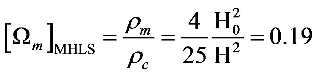
We briefly summarize the main experimental results relevant for this work. The matter density of the universe is given by [2,3]:
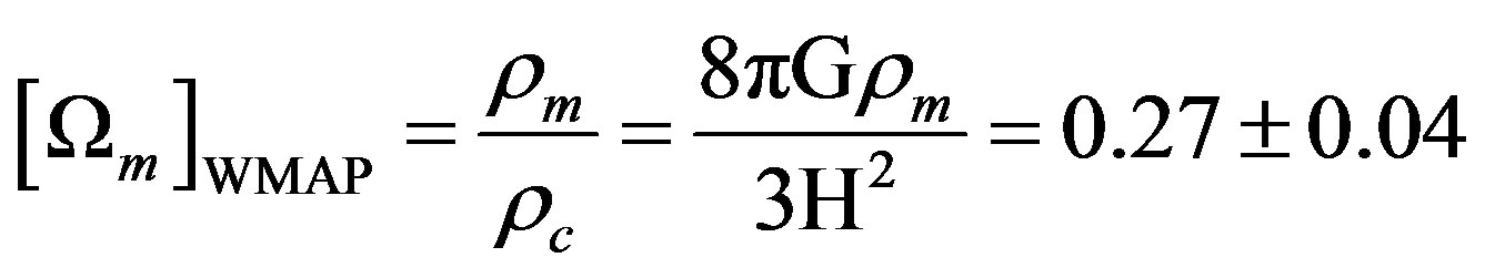 , (2)
, (2)
rm is the matter density, which includes baryonic as well as dark matter (DM). The critical density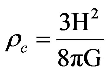
depends on the value of the Hubble constant H and G is Newton’s gravitational constant. The baryonic density is estimated to be about 16% of the total matter density, the rest is matter in some other form. The value of the baryonic density is inferred from the observed primordial abundance of elements formed in the early universe [3-5]. The total matter density in Equation (2) is obtained from gravitational effects on the motion of stellar objects. We will not discuss any further about this distinction and in our work we will derive the total density including dark and non-dark matter. A contribution to the density is due to relativistic particles, especially neutrinos and photons; their contribution is presently small and we will neglect it [2,3].
Observations and detailed calculations reveal that some form of energy is missing which suggested an “ad hoc” potential term:
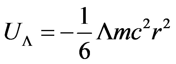 , (3)
, (3)
 is the cosmological constant first introduced by A. Einstein [3]. Even though we are using Newtonian cosmology in Equation (3) and in the following, the results remain unchanged when general relativity is used. The cosmological constant was first introduced with the desire of obtaining stationary solutions for the universe, a concept that turned out to be incorrect after Hubble’s observations. Nevertheless, experimental data forced to include a form of unknown energy exemplified by Equation (3) and dubbed as: Dark Energy (DE). The experimental value of the DE density, and implicitly of the cosmological constant Λ is [2]:
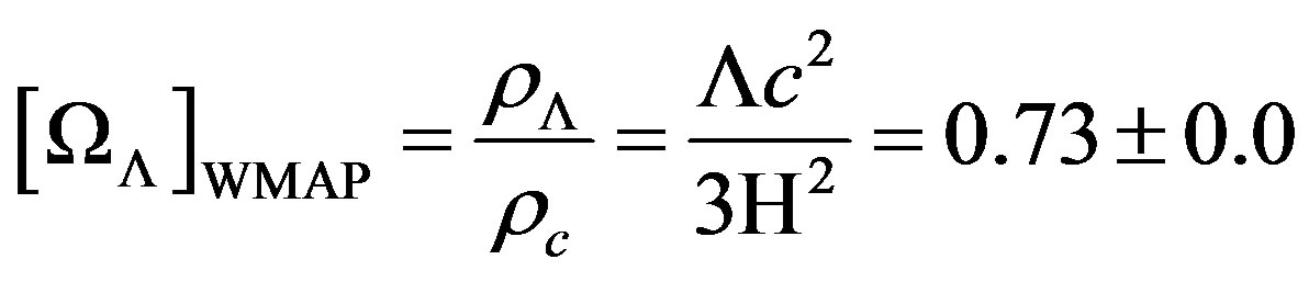 . (4)
. (4)
Equations (2) and (4) give the total density (neglecting the small contribution from relativistic particles):
 . (5)
. (5)
The model described above is known as theΛCDM: it includes the cosmological constant Λ and DM [3]. Since the Λ constant is positive, Equation (3) results in an acceleration: galaxies might be accelerating from each other at large distances, instead of decelerating, as one would naively expect from Newtonian’s gravitational law. Most of nowadays theoretical and experimental efforts are concentrating on determining the nature of DM and DE. In this paper we will show that a simple modification of Hubble’s law (MHL), can explain the experimental results without the need of invoking any DE as given in Equation (3).
2. The Modified Hubble’s Law
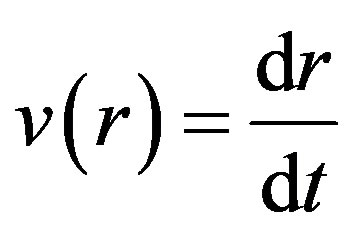
There is no reason why Hubble’s law given in Equation (1) should be valid for any value of the distance r. In particular it is already assumed in Equation (1) that when r à 0, v à 0. A constant term could be added which might not be in contrast with actual experimental data. Such a term is usually neglected, in agreement with Equation (1), and we will conform to such an assumption. The major problem arises when distances become very large. Physically, we do not expect velocities to diverge linearly. In particular, because of total energy conservation, we expect HL to be modified at large r. To take these features into account we propose an expansion of the velocity as:
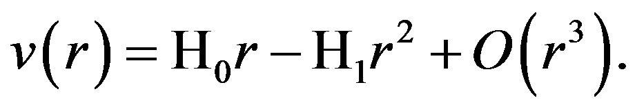 (6)
(6)
In Figure 1, we plot the velocity of galaxies versus their relative distances as reported from the Hubble Space Telescope (HST) collaboration [2], full dots. In the same figure we display a linear fit according to HL (Equation (1)—full line), and a second order expansion (Equation (6)—dashed line). Clearly the MHL reproduces the data better in particular at large distances. The inclusion of even higher order terms is not justified by the available data, but it might be important if measurements at larger distances will be available in the future. Notice the small difference between the values of the constants H and H0 in the two approximations. The value of H1 is relatively small, and so is the correction to HL, which suggests that Equation (1) is valid in first approximation, thus we expect fluctuations to be small in agreement to data.
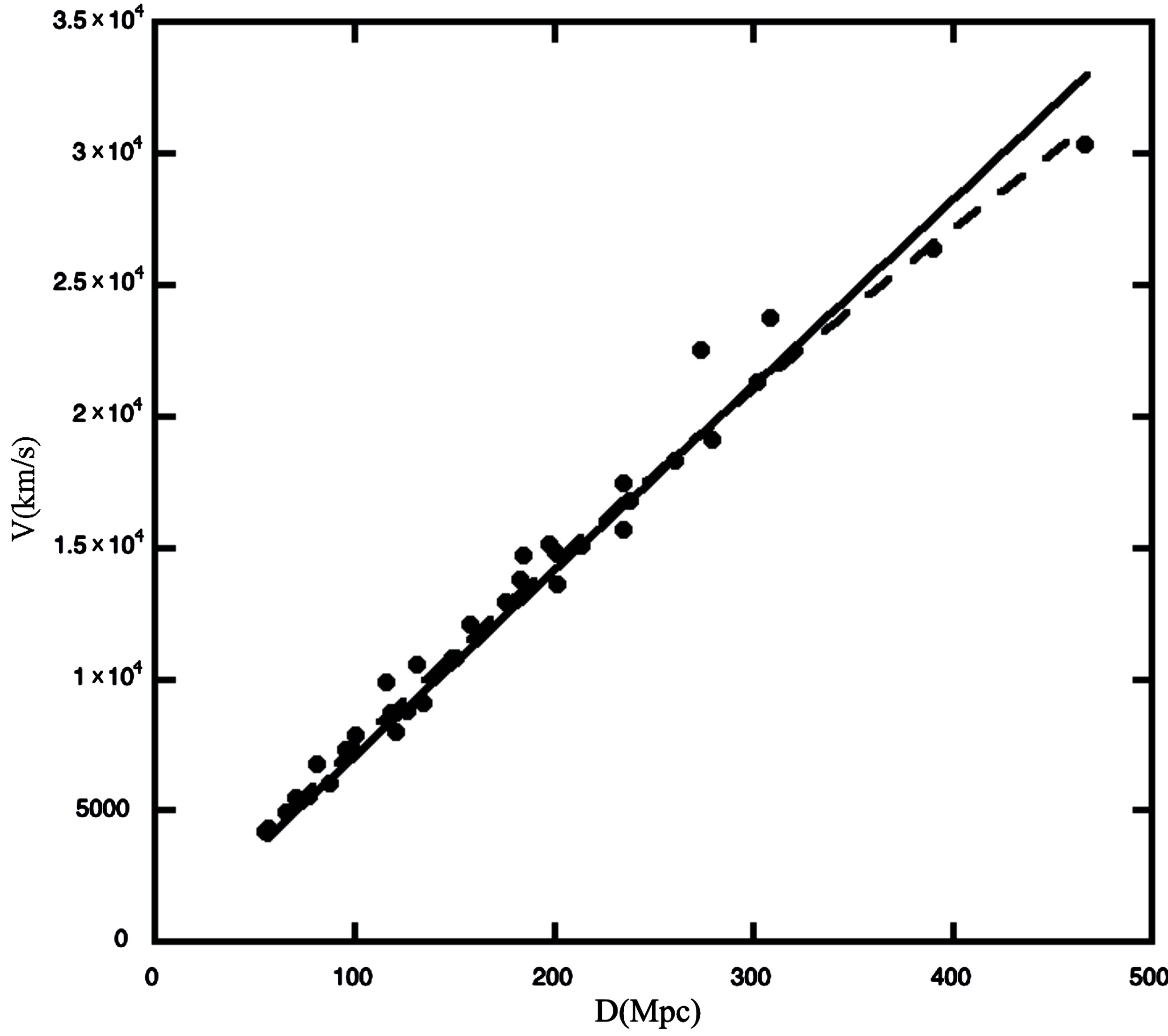
Figure 1. Velocity-distance plot. The data (full circles) are from reference [2]. The full line is a fit according to Hubble’s law [1] (H = 70.6 km·s–1Mpc–1 = 2.310–18·s–1), while the dashed line takes into account second order corrections, resulting in a better reproduction of the data (H0 = 76.9 km·s–1Mpc–1 = 2.410–18·s–1 and H1 = 0.022 km·s–1Mpc–2 = 2.310–44 m–1·s–1).
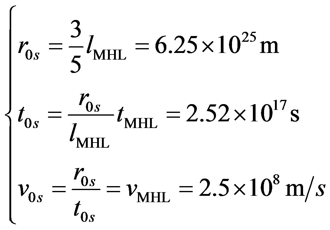
From the value of the constants in the MHL, we can define a typical time, distance, velocity and acceleration:
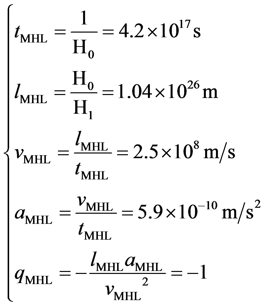 (7)
(7)
The last quantity in Equation (7), is the “deceleration parameter” [2,3] which should be compared to the experimental value at present time:
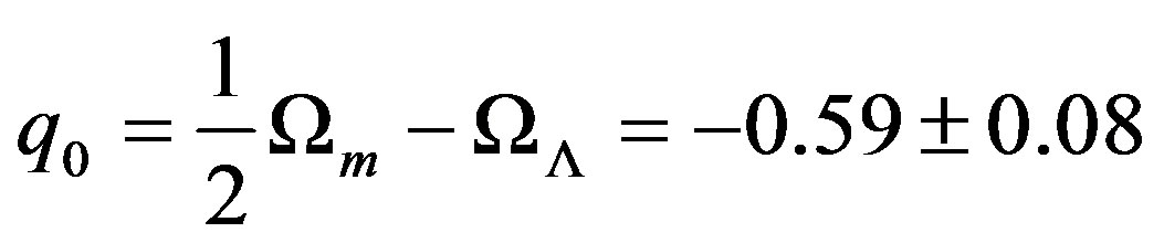 . (8)
. (8)
The difference with our estimate is due to the role of the gravitational attraction, which would favour a positive value of the deceleration parameter. It is a simple exercise [3] to show that for a purely gravitational system
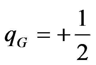 , when the total energy of the system is zero (flat universe). Just by naively adding the Big-Bang contribution, Equation (7) and the gravitational contribution, qG, we get a deceleration value very close to the experiments within the experimental error. However, the deceleration parameter depends on the universe radius at present time, as we will discuss below. Equation (8) supports the possibility of Dark Energy [2,3].
The quantities in Equation (7) represent the limit of validity of our approach since v(lMHL) = 0 from Equation (6). Notice that the farthest distance measured and plotted in Figure 1 is Dmax = 1.4×1025 m, well below the value in Equation (7). Thus our considerations will be valid for distances of the order of lMHL. Future data at larger distances might put more firm constraints. The apparently innocent modification of the HL has dramatic consequences, as we will demonstrate in a simple “dust” model of the universe [3].
A spherical shell of mass m and radius r expands with velocity v. The total mass within the shell is given by M. Let us define the total energy per unit mass as: ε = E/m. It is given by [3]:
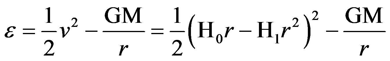 , (9)
, (9)
where we used the MHL, Equation (6). We notice that the experimental result, Equation (5), implies ε = 0 and the universe is flat [2,3].
The appearance of higher order terms in Equation (9), suggests the possibility that the universe might expand and finally reach an equilibrium position r0s. This equilibrium position can be calculated from the first derivative of Equation (9):
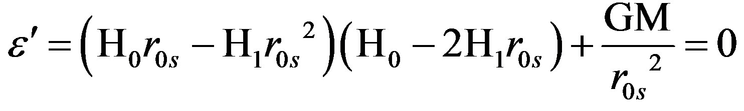 , (10a)
which gives:
 . (10b)
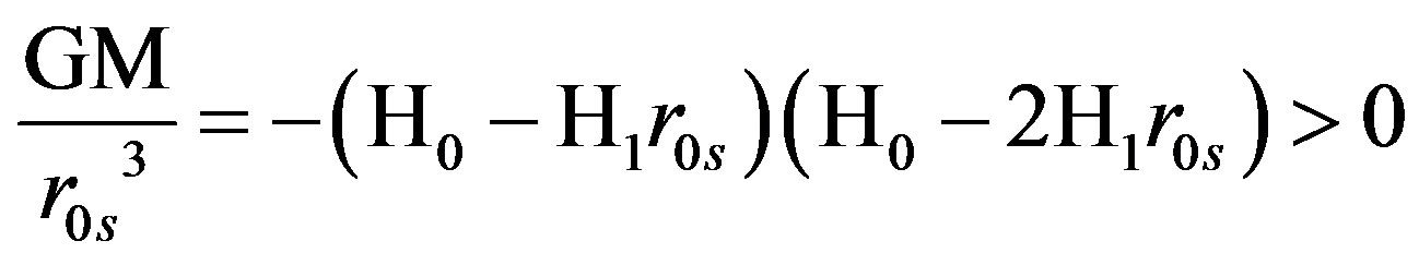
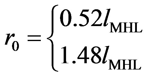
Since the mass must be positive, the range of equilibrium values, which satisfy Equations (10a) and (10b), is rather restricted: 0.5 < r0s/lH < 1. Assuming a flat universe, ε = 0, gives the values:
 (11)
(11)
which is the equilibrium value of the radius of the universe to be reached approximately at time t0s. The first derivative of Equation (10a) calculated at r0s reveals that the equilibrium solution is a maximum thus unstable. After reaching r0s, the fate of the universe will be determined by fluctuations: either collapse or expand forever!
From r0s we can estimate the total density of the universe (both dark and baryonic density) at time t0s:
 . (12)
where we have used Equations (2) and (10a) and (10b) and we have taken into account the small difference between the Hubble’s constants obtained using Equations (1) and (6). The calculated value of the density is not too far away from the experimental value, Equation (2), but it is definitely outside the quoted error. This suggests that the possibility of reaching an unstable equilibrium solution (even though at later times) might not be supported by the data. Other possibilities are that the universe has not expanded enough to reach r0s or that it has already expanded above r0s and it will never stop.
Before proceeding further, it is instructive to estimate the value of the DE using Equation (9). Recall that in the ΛCDM approach, the energy per unit mass is given by:
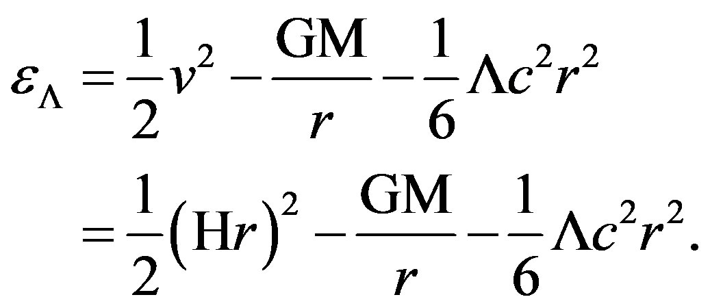 (13)
(13)
It is evident from Equation (13) that the particular choice of the cosmological potential is to balance the kinetic part coming from the HL. Imposing ε(r0s) = εL(r0s) gives:
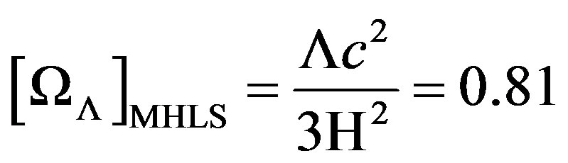 . (14)
The estimated value is again not too different from the experimental value given in Equation (4) but definitely outside the experimental error. Notice that Equation (5) is fulfilled in the model case. Before discussing under which conditions the data can be reproduced we must stress that in our model there is no need for dark-energy, thus Λ = 0. This is an important consequence of the modification introduced in Equation (6): the extra energy needed to reproduce the experimental data is due to the kinetic component and not to the potential one as assumed in Equations (3) and (13).
We can reverse the arguments above and, starting from the experimental value of the matter density, derive the value of the radius of the universe at present time. Assuming a stationary solution, we can derive the value of r0s, which corresponds to the experimental density, Equation (2). Using Equations (10a), (12) and (2), it is a simple exercise to show that the experimental value of the matter density does not support a stationary solution at present time even for ε ≠ 0. Alternatively, assuming a flat universe, ε = 0, we can derive the matter density from Equation (9) and put it equal to the experimental value. This gives solutions for the radius of the universe at present time (the age of the universe). Since Equation (9) is quadratic in r we get two values:
 (15)
(15)
Notice that the smaller solution in Equation (15) is not too much different from the stationary solution, Equation (11). If this lower value is the actual radius of the universe, then the universe will expand and eventually reach the (unstable) equilibrium solution given in Equation (11). The age of the universe corresponding to such r0 is:
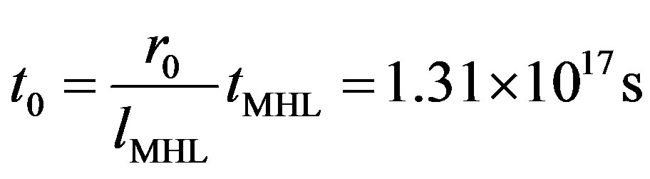 , a little smaller than the equilibrium value t0s. The larger r0 value in Equation (15) is near the limits of validity of our approach given in (7). If a larger value than r0s, would be supported from the data, we could conclude that the universe has reached the unstable equilibrium position and, because of fluctuations, will continue to expand forever. The age of the universe corresponding to the larger r0 value is t0 = 3.73 × 10¹⁷ s, close to the quoted value 4.34 × 10¹⁷ s [2,3], obtained from the inverse of the Hubble’s constant H. Such an age value would support a universe expanding forever. Finally, using Equation (15) to derive the DE density from Equations (13) and (9), reproduces the experimental value given in Equation (4) as expected.
It is instructive to recover these results starting from the Friedmann equation from general relativity. Using the same formalism as in ref. [3] (Equation (29.114)), the Friedmann equation, is written as:
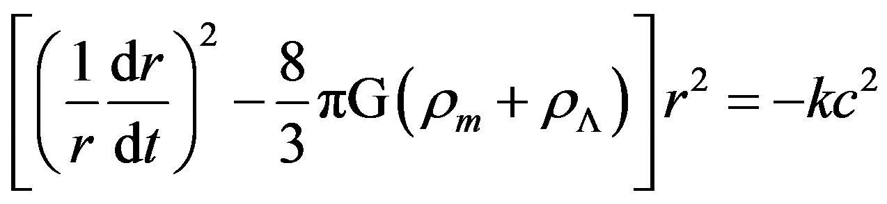 . (16)
The latter equation is the equivalent of the Newtonian Equation (9) where the role of the energy is taken by the space curvature k. The density due to relativistic particles has been neglected since its contribution is small. Since,
 , using the linear Hubble’s law and the density values given in Equations (2) and (4) gives k = 0, i.e. a flat universe. If we now substitute the MHL, Equation (6), into Equation (16) and neglect the Dark Energy term, we obtain:
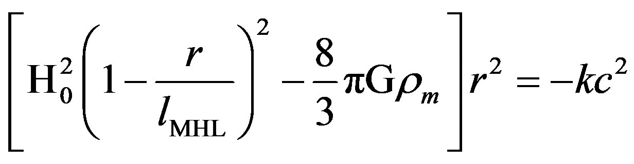 . (17)
Putting r = r0, Equation (15), and taking into account the small difference between H and H0, gives k = 0. Again the role of the DE has been taken by the correction in the kinetic part in agreement to the experimental data plotted in Figure 1.
An important signature for DE is attributed to the deceleration parameter, which is negative at present time, Equation (8). From the velocity distribution, Equation (6), we can derive the acceleration distribution by taking the derivative respect to time: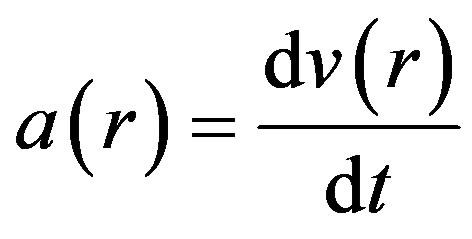 . Thus, the deceleration parameter is:
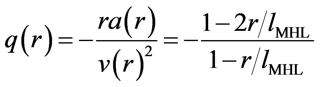 . (18)
Averaging Equation (18) over the radius of the universe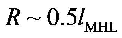 , gives:
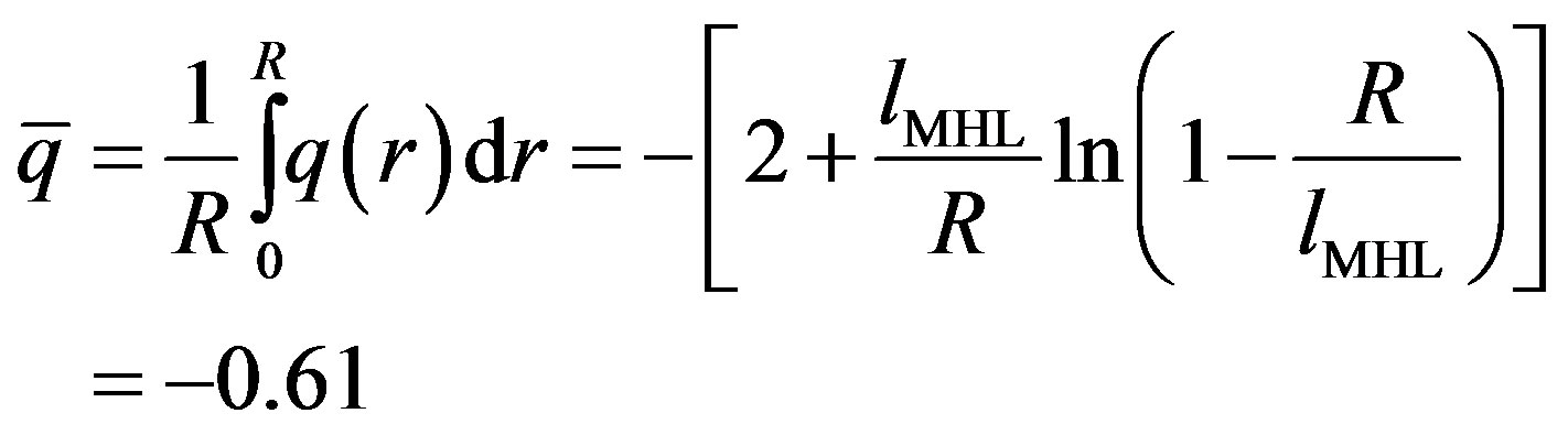 (19)
(19)
This estimate agrees with experiments, Equation (8). The average deceleration parameter changes sign when the radius of the universe , thus excluding the second possible solution in Equation (15). In contrast to Equation (18), the linear Hubble law, Equation (1), gives q = –1, independent on the radius of the universe. The result above is obtained from the time derivative of the velocity distribution. The origin of such an acceleration distribution (as well as the velocity distribution displayed in Figure 1) might be due to a combination of gravitational effects and DE, or to gravitational instabilities and initial conditions from the Big-Bang [6]. These instabilities might be responsible for fluctuations in the velocity distribution of galaxies which result in important deviations from Hubble’s law, Equation (1) and its modification, Equation (6), proposed in this work [7,8]. The importance of Equation (19) is to exclude the larger radius solution in Equation (15), while Equation (9) does not require any DE.
In conclusion, in this work we have shown that higher order corrections to Hubble’s law have important consequences and that there is no need for the dark energy, thus the cosmological constant Λ = 0. The role of the dark energy is played by higher order corrections to the kinetic energy. We have estimated the value of the matter density (both baryonic and not) assuming the possibility that the universe will eventually reach an unstable equilibrium. The unstable equilibrium could be obtained if the present value of the radius of the universe is about 5.4 × 1025 m. On the other hand if the present value of the radius of the universe is larger than 6.25 × 1025 m, i.e. above the equilibrium point, then the universe will expand forever. The universe is presently accelerating at a rate lower than the initial Big-Bang acceleration due to the gravitational attraction. The deceleration parameter suggests that the universe has not reached the unstable equilibrium point yet, thus supporting the smaller value of the radius of the universe, Equation (15). Because of the sensitivity of our results to the data we do not exclude the possibility that further measurements of the velocity of recessions of galaxies as function of the distance will give more constraints on the polynomial expansion proposed in this work. In particular we need measurements at larger distances than reported in Figure 1. Finally, preliminary calculations in the framework of general relativity are in agreement with the results discussed here and we will discuss them in detail in a future publication.
REFERENCES
- E. Hubble, “A Relation between Distance and Radial Velocity among Extra-Galactic Nebulae,” The Proceedings of the National Academy of Sciences, Vol. 15, No. 3, 1929, pp. 168-173. doi:10.1073/pnas.15.3.168
- A. G. Riess, et al., “New Hubble Space Telescope Discoveries of Type Ia Supernovae at z ≥ 1: Narrowing Constraints on the Early Behavior of Dark Energy,” The Astrophysical Journal, Vol. 659, No. 1, 2007, pp. 98-121. doi:10.1086/510378
- B. W. Carroll and D. A. Ostlie, “An Introduction to Modern Astrophysics,” 2nd Edition, Addison-Wesley, San Francisco, 2007.
- A. Bonasera, Y. El Masri and J. B. Natowitz, “An Introduction to Modern Nuclear Science and Its Applications,” Taylor & Francis Group Books, Inc., 2013.
- D. N. Schramm and M. S. Turner, “Big-Bang Nucleosynthesis Enters the Precision Era,” Reviews of Modern Physics, Vol. 70, No. 1, 1998, pp. 303-318. doi:10.1103/RevModPhys.70.303
- H. G. Schuster, “Deterministic Chaos,” VCH-Editor, Weinheim, 1995.
- M. S. Roberts and M. P. Haynes, “Physical Parameters Along the Hubble Sequence,” Annual Review of Astronomy and Astrophysics, Vol. 32, 1992, pp. 115-152. doi:10.1146/annurev.aa.32.090194.000555
- E. Komatsu, et al., “WMAP Collaboration,” The Astrophysical Journal Supplement Series, Vol. 192, No. 2, 2011, p. 18.
NOTES
*In loving memory of my son Luca (1992-2012).