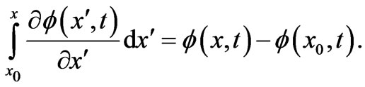
Journal of Modern Physics
Vol.2 No.11(2011), Article ID:8629,22 pages DOI:10.4236/jmp.2011.211156
Beyond the Dirac Phase Factor: Dynamical Quantum Phase-Nonlocalities in the Schrödinger Picture
Department of Physics, University of Cyprus, Nicosia, Cyprus
E-mail: cos@ucy.ac.cy
Received June 10, 2011; revised July 19, 2011; accepted July 28, 2011
Keywords: Aharonov-Bohm, Gauge Transformations, Dirac Phase Factor, Quantum Phases
ABSTRACT
Generalized solutions of the standard gauge transformation equations are presented and discussed in physical terms. They go beyond the usual Dirac phase factors and they exhibit nonlocal quantal behavior, with the well-known Relativistic Causality of classical fields affecting directly the phases of wavefunctions in the Schrödinger Picture. These nonlocal phase behaviors, apparently overlooked in path-integral approaches, give a natural account of the dynamical nonlocality character of the various (even static) Aharonov-Bohm phenomena, while at the same time they seem to respect Causality. For particles passing through nonvanishing magnetic or electric fields they lead to cancellations of Aharonov-Bohm phases at the observation point, generalizing earlier semiclassical experimental observations (of Werner & Brill) to delocalized (spread-out) quantum states. This leads to a correction of previously unnoticed sign-errors in the literature, and to a natural explanation of the deeper reason why certain time-dependent semiclassical arguments are consistent with static results in purely quantal Aharonov-Bohm configurations. These nonlocalities also provide a remedy for misleading results propagating in the literature (concerning an uncritical use of Dirac phase factors, that persists since the time of Feynman’s work on path integrals). They are shown to conspire in such a way as to exactly cancel the instantaneous Aharonov-Bohm phase and recover Relativistic Causality in earlier “paradoxes” (such as the van Kampen thought-experiment), and to also complete Peshkin’s discussion of the electric Aharonov-Bohm effect in a causal manner. The present formulation offers a direct way to address time-dependent singlevs double-slit experiments and the associated causal issues—issues that have recently attracted attention, with respect to the inability of current theories to address them.
1. Introduction
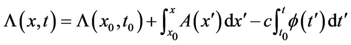
The Dirac phase factor—with a phase containing spatial or temporal integrals of potentials (of the general form )—is the standard and widely used solution of the gauge transformation equations of Electrodynamics (with A and
  vector and scalar potentials respectively). In a quantum mechanical context, it connects wavefunctions of two systems (with different potentials) that experience the same classical fields at the observation point (r, t), the two more frequently discussed cases being: either systems that are completely gauge-equivalent (a trivial case with no physical consequences), or systems that exhibit phenomena of the Aharonov-Bohm type (magnetic or electric) [1]—and then this Dirac phase has nontrivial observable consequences (mathematically, this being due to the fact that the corresponding “gauge function” is now multiplevalued). In the above two cases, the classical fields experienced by the two (mapped) systems are equal at every point of the accessible spacetime region. However, it has not been widely realized that the gauge transformation equations, viewed in a more general context, can have more general solutions than simple Dirac phases, and these lead to wavefunction-phase-nonlocalities that have been widely overlooked and that seem to have important physical consequences. These nonlocal solutions are applicable to cases where the two systems are allowed to experience different fields at spacetime points (or regions) that are remote to (and do not contain) the observation point (r, t) (these regions being physically accessible to the particle, unlike genuine Aharonov-Bohm cases). In this article we rigorously show the existence of these generalized solutions, demonstrate them in simple physical examples, and fully explore their structure, presenting cases (and closed analytical results for the wavefunction-phases) that actually connect (or map) two quantal systems that are neither physically equivalent nor of the usual Aharonov-Bohm type. We also fully investigate the consequences of these generalized (nonlocal) influences (on wavefunction-phases) and find them to be numerous and important; we actually find them to be of a different type in static and in time-dependent field-configurations (and in the latter cases we show that they lead to Relativistically causal behaviors, that apparently resolve earlier “paradoxes” arising in the literature from the use of standard Dirac phase factors). The nonlocal phase behaviors discussed in the present work may be viewed as a justification for the (recently emphasized [2]) terminology of “dynamical nonlocalities” associated with all Aharonov-Bohm effects (even static ones), although in our approach these nonlocalities seem to also respect Causality (without the need to independently invoke the Uncertainty Principle)—and, to the best of our knowledge, this is the first theoretical picture with such characteristics.
In order to introduce some background and further motivation for this article let us first remind the reader of a very basic property that will be central to everything that follows, which however is usually taken to be valid only in a restricted context (but is actually more general than often realized). This property is a simple (U(1)) phase-mapping between quantum systems, and is usually taken in the context of gauge transformations, ordinary or singular; here, however, it will appear in a more general framework, hence the importance of reminding of its independent, basic and more general origin. We begin by recalling that, if  and
and  are solutions of the time-dependent Schrödinger (or Dirac) equation for a quantum particle of charge q that moves (as a test particle) in two distinct sets of (predetermined and classical) vector and scalar potentials (
 ) and (
 ), that are generally spatiallyand temporally-dependent [and such that, at the spacetime point of observation (r, t), the magnetic and electric fields are the same in the two systems], then we have the following formal connection between the solutions (wavefunctions) of the two systems
 (1)
(1)
with the function  required to satisfy
 (2)
(2)
The above property can be immediately proven by substituting each  into its corresponding (ith) timedependent Schrödinger equation (namely with the set of potentials (
 ,
, ): one can then easily see that (1) and (2) guarantee that both Schrödinger equations are indeed satisfied together (after cancellation of a few terms and then elimination of a global phase factor in system 2). [In addition, the equality of all classical fields at the observation point, namely

for the magnetic fields and

for the electric fields, is obviously consistent with all Equations (2) (as is easy to see if we take the curl of the 1st and the grad of the 2nd)—provided, at least, that  is such that interchanges of partial derivatives with respect to all spatial and temporal variables (at the point (r, t)) are allowed].
As already mentioned, the above fact is of course well-known within the framework of the theory of quantum mechanical gauge transformations (the usual case being for , hence for a mapping from a system with no potentials); but in that framework, these transformations are supposed to connect (or map) two physically equivalent systems (more rigorously, this being true for ordinary gauge transformations, in which case the function
 , the so-called gauge function, is unique (single-valued) in spacetime coordinates). In a formally similar manner, the above argument is also often used in the context of the so-called “singular gauge transformations”, where
  is multiple-valued, but the above equality of classical fields is still imposed (at the observation point, which always lies in a physically accessible region); then the above simple phase mapping (at all points of the physically accessible spacetime region, that always and everywhere experience equal fields) leads to the standard phenomena of the Aharonov-Bohm type, where unequal fields in physically inaccessible regions have observable consequences. However, we should keep in mind that that above property ((1) and (2) taken together) can be more generally valid—and in this article we will present cases (and closed analytical results for the appropriate phase connection
 ) that actually connect (or map) two systems (in the sense of (1)) that are neither physically equivalent nor of the usual Aharonov-Bohm type. And naturally, because of the above provision of field equalities at the observation point, it will turn out that any nonequivalence of the two systems will involve remote (although physically accessible) regions of spacetime, namely regions that do not contain the observation point (r, t) (and in which regions, as we shall see, the classical fields experienced by the particle may be different in the two systems).
2. Motivation
One may wonder on the actual reasons why one should be looking for more general cases of a simple phase mapping of the type (1) between nonequivalent systems. To answer this, let us take a step back and first recall some simple and well-known results that originate from the above phase mapping. It is standard knowledge, for example, that, if we want to find solutions  of the t-dependent Schrödinger (or Dirac) equation for a quantum particle (of charge q) that moves along a (generally curved) one-dimensional (1-D) path, and in the presence (somewhere in the embedding 3-dimensional (3-D) space) of a fairly localized (and time-independent) classical magnetic flux
  that does not pass through any point of the path, then we formally have
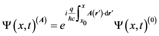 (3)
(3)
(the dummy variable r' describing points along the 1-D path, and the term “formally” signifying that the above is valid before imposition of any boundary conditions (meaning that these are to be imposed only on  and not necessarily on
![]() ). In (3),
). In (3),  is a formal solution of the same system in the case of absence of any potentials (hence with magnetic flux
  everywhere in the 3-D space). The above holds because, for all points r' of the 1-D path, the particle experiences a vector potential
  of the form
  (since the magnetic field is
  for all r', by assumption), in combination with the above phase-mapping (with a phase
 ) between two quantum systems, one in the presence and one in the absence of a vector potential (i.e. the potentials in (2) being
  and
and , together with
  if we decide to attribute everything to vector potentials only). In this particular system, the obvious
  that solves the above
  (for all points of the 1-D space available to the particle) is indeed

(since ), and this gives (3)
(if r denotes the above point x of observation and ![]() the arbitrary initial point
the arbitrary initial point  (both lying on the physical path), and if the constant
  is taken to be zero).
What if, however, some parts of the magnetic field that comprise the magnetic flux  actually pass through some points or a whole region (interval) of the path available to the particle? In such a case, the above standard argument is not valid (as A cannot be written as a grad at any point of the interval where the magnetic field
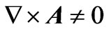 ). Are there however general results that we can still write for
 , if the spatial point of observation x is again outside the interval with the nonvanishing magnetic field? Or, what if in the previous problems, the magnetic flux (either remote, or partly passing through the path) is time-dependent
 ? (In that case then, there exists in general an additional electric field E induced by Faraday’s law of Induction on points of the path, and the usual gauge transformation argument is once again not valid).
Returning to another standard (solvable) case (which is actually the “dual” or the “electric analog” of the above), if along the 1-D physical path the particle experiences only a spatially-uniform (but generally time-dependent) classical scalar potential , we can again formally map
  to a potential-free solution
 through a
  that now solves
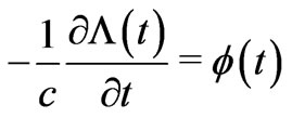 , and this gives
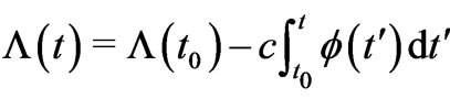 , leading to the “electric analog” of (3), namely
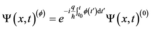 (4)
(4)
with obvious notation. (Notice that, for either of the two mapped systems in this problem, the electric field is zero at all points of the path). What if, however, the scalar potential has also some x-dependence along the path (that leads to an electric field (in a certain interval) that the particle passes through)? In such a case, the above standard argument is again not valid. Are there however general results that we can still write for , if the spatial point of observation x is again outside the interval with the nonvanishing electric field?
We state here directly that this article will provide affirmative answers to questions of the type posed above, by actually giving the corresponding general results in closed analytical forms.
At this point it is also useful to briefly reconsider the earlier mentioned case, namely of a time-dependent  that is remote to the 1-D physical path, because in this manner we can immediately provide another motivation for the present work: this time-dependent problem is surrounded with a number of important misconceptions in the literature (the same being true about its electric analog, as we shall see): the formal solution that is usually written down for a
  is again (3), namely the above spatial line integral of A, in spite of the fact that A is now t-dependent; the problem then is that, because of the first of (2),
  must now have a t-dependence and, from the second of (2), there must necessarily be scalar potentials involved in the problem (which have been by force set to zero, in our pre-determined mapping between vector potentials only). Having decided to use systems that experience only vector (and not scalar) potentials, the correct solution cannot be simply a trivial t-dependent extension of (3). A corresponding error is usually made in the electric dual of the above, namely in cases that involve r-dependent scalar potentials, where (4) is still erroneously used (with
  replaced by
 ), giving an r-dependent
 , although this would necessarily lead to the involvement of vector potentials (through the first of (2) and the r-dependence of
 ) that have been neglected from the beginning – a situation (and an error) that appears, in exactly this form, in the description of the so-called electric Aharonov-Bohm effect [1,3] as we shall see.
Speaking of errors in the literature, it might here be the perfect place to also point to the reader the most common misleading statement often made in the literature (and again, for notational simplicity, we restrict our attention to a one-dimensional system, with spatial variable x, although the statement is obviously generalizable to (and often made for systems of) higher dimensionality by properly using line integrals over arbitrary curves in space): It is usually stated [e.g. in Brown & Holland [4], see i.e. their Equation (57) applied for vanishing boost velocity v = 0] that the general gauge function that connects (through a phase factor ) the wavefunctions of a quantum system with no potentials (i.e. with a set of potentials
 ) to the wavefunctions of a quantum system that moves in vector potential
  and scalar potential
  (i.e. in a set of potentials
 ) is the obvious combination (and a natural extension) of (3) and (4), namely
 (5)
(5)
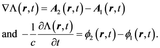
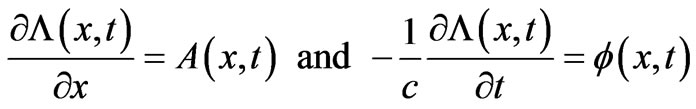
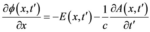
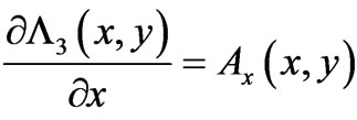
which, however, is incorrect for x and t uncorrelated variables: it does not satisfy the standard system of gauge transformation equations
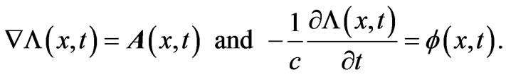 (6)
(6)
The reader can easily see why: 1) when the  operator acts on Equation (5), it gives the correct
  from the 1st term, but it also gives some annoying additional nonzero quantity from the 2nd term (that survives because of the x-dependence of
 ); hence it invalidates the first of the basic system (6). 2) Similarly, when the
 operator acts on Equation (5), it gives the correct
 from the 2nd term, but it also gives some annoying additional nonzero quantity from the 1st term (that survives because of the t-dependence of A); hence it invalidates the second of the basic system (6). It is only when A is t-independent, and
  is spatially-independent, that Equation (5) can be correct (as the above annoying terms do not appear and the basic system is satisfied), although it is still not necessarily the most general form for
 , as we shall see. [An alternative form that is also widely thought to be correct is again Equation (5), but with the variables that are not integrated over implicitly assumed to belong to the initial point (hence a
 ![]() replaces t in A, and simultaneously an
replaces t in A, and simultaneously an  replaces x in
 ). However, one can see again that the system (6) is not satisfied (the above differential operators, when acted on
 , give
  and
and , hence not the values of the potentials at the point of observation
  as they should), this not being an acceptable solution either].
What is the problem here? Or, better put, what is the deeper reason for the above inconsistencies? The short answer is the uncritical use of Dirac phase factors that come from path-integral treatments. It is indeed obvious that the form (5) that is often used in the literature in canonical (non-path-integral) formulations where x and t are uncorrelated variables (and not correlated to produce a path ) is not generally correct, and that is one of the main points that has motivated this work. We will find generalized results that actually correct Equation (5) through extra nonlocal terms, and through the proper appearance of
  and
and ![]() (as in Equation (11) and Equation (12) to be found later in Section 3), and these are the exact ones (namely the exact
(as in Equation (11) and Equation (12) to be found later in Section 3), and these are the exact ones (namely the exact  that at the end, upon action of
  and
and  satisfies exactly the basic system (6), viewed as a system of Partial Differential Equations (PDEs)). And the formulation that gives these results is generalized later in the article, for
  (in the 2-D static case) and also for
  (in the full dynamical 2-D case), and leads to the exact (nontrivial) forms of the phase function
  that satisfy (in all cases) the system (6)—with the direct verification (i.e. proof, by “going backwards”, that these forms are indeed the exact solutions of (6)) also being given for the reader’s convenience. [For the “direct” and rigorous mathematical derivations see [5].]
This article gives a full exploration of issues related to the above motivating discussion, by pointing to a “practical” (and generalized) use of gauge transformation mapping techniques, that at the end lead to these generalized (and, at first sight, unexpected) solutions for the general form of . For cases such as the ones discussed above, or even more involved ones, there still appears to exist a simple phase mapping (between two inequivalent systems), but the phase connection
  seems to contain not only integrals of potentials, but also “fluxes” of the classical field-differences from remote spacetime regions (regions, however, that are physically accessible to the particle). The above mentioned systems are the simplest ones where these new results can be applied, but apart from this, the present investigation seems to lead to a number of nontrivial corrections of misleading (or even incorrect) reports of the above type in the literature, that are not at all marginal (and are due to an incorrect use of a path-integral viewpoint in an otherwise canonical framework—an error that appears to have been made repeatedly since the original conception of the path-integral formulation, as we shall see). The generalized
  -forms also lead to an honest resolution of earlier “paradoxes” (involving Relativistic Causality), and in some cases to a new interpretation of known semiclassical experimental observations, corrections of certain sign-errors in the literature, and nontrivial extensions of earlier semiclassical results to general (even completely delocalized) states. [As a byproduct, we will also show that—contrary to what is usually stated in earlier but also recent popular reports—the semiclassical phase picked up by classical trajectories (that are deflected by the Lorentz force) is opposite (and not equal) to the so-called Aharonov-Bohm phase due to the flux enclosed by the same trajectories; we will also provide 2 figures to visually assist the detailed proof of this result as well as to facilitate an elementary physical understanding of this opposite sign relation]. Most importantly, however, the new formulation seems capable of addressing causal issues in time-dependent singlevs double-slit experiments, an area that seems to have recently attracted attention [2, 6,7]).
3. 1-D Dynamic Case
Let us begin with the simplest case of 1-D systems but in the most general dynamic environment, i.e. a single quantum particle of charge q, but in the presence of arbitrary (spatially nonuniform and time-dependent) vector and scalar potentials. Let us actually consider this particle moving either inside a set of potentials  and
and  (case 1) or inside a set of potentials
  and
and  (case 2), and try to determine the most general gauge function
  that takes us from (maps) the wavefunctions of the particle in case 1 to those of the same particle in case 2 (meaning the usual mapping (1) between the wavefunctions of the two systems through the phase factor
 ). [As already noted, we should keep in mind that for this mapping to be possible we must assume that at the point
  of observation (or “measurement” of
  or the wavefunction
 ) we have equal electric fields (
 )namely
 (7)
(7)
(so that the A’s and ’s in (7) can indeed satisfy the basic system of Equations (2), or equivalently, of the system of equations (10) below—as can be seen by tak ing the
  of the 1st and the
  of the 2nd of the system (10) and adding them together). But again, we will not exclude the possibility of the two systems passing through different electric fields in other regions of spacetime (that do not contain the observation point), i.e. for
 . In fact, this possibility will come out naturally from a careful solution of the basic system (10); it is for example straightforward for the reader to immediately verify that the results (11) or (12) that will be derived below (and will contain contributions of electric field-differences from remote regions of spacetime) indeed satisfy the basic input system of Equations (10), something that will be explicitly verified below].
Returning to the question on the appropriate  that takes us from the set
  to the set
 , we note again that, in cases of static vector potentials (
 ’s) and spatially uniform scalar potentials (
 ’s) the form usually given for
  is the well-known
 (8)
(8)
with  and
and  (and it can be viewed as a combination of (3) and (4), being immediately applicable to the description of cases of combined magnetic and electric Aharonov-Bohm effects).
But as already noted, even in the most general case, with t-dependent A’s and x-dependent ’s (and with the variables x and t being completely uncorrelated), it is often stated in the literature that the appropriate
  has a form that is a plausible extention of (8), namely
 (9)
(9)
[with Equation (57) of Ref. [4], taken for v = 0, being a very good example to point to, since that article does not use a path-integral language, but a canonical formulation with uncorrelated variables]. And as already pointed out in Section 2, this form is certainly incorrect for uncorrelated variables x and t (the reader can easily verify that the system of Equations (10) below is not satisfied by (9) —see again Section 2, especially the paragraph after Equation (6)). We will find in the present work that the correct form consists of two major modifications of (9): 1) The first leads to the natural appearance of a path that continuously connects initial and final points in spacetime, a property that (9) does not have [indeed, if the integration curves of (9) are drawn in the  -plane, they do not form a continuous path from
  to
to ]. 2) And the second modification is highly nontrivial: it consists of nonlocal contributions of classical electric field-differences from remote regions of spacetime. We will discuss below the consequences of these terms and we will later show that such nonlocal contributions also appear (in an extended form) in more general situations, i.e. they are also present in higher spatial dimensionality (and they then also involve remote magnetic fields in combination with the electric ones); these lead to modifications of ordinary Aharonov-Bohm behaviors or have other important consequences, one of them being a natural remedy of Causality “paradoxes” in time-dependent Aharonov-Bohm experiments.
The form (9) commonly used is of course motivated by the well-known Wu & Yang [8] nonintegrable phase factor, that has a phase equal to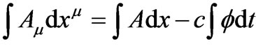 a form that appears naturally within the framework of path-integral treatments, or generally in physical situations where narrow wavepackets are implicitly assumed for the quantum particle: the integrals appearing in (9) are then taken along particle trajectories (hence spatial and temporal variables not being uncorrelated, but being connected in a particular manner
  to produce the path; all integrals are therefore basically only time-integrals). But even then, Equation (9) is valid only when these trajectories are always (in time) and everywhere (in space) inside identical classical fields for the two (mapped) systems. Here, however, we will be focusing on what a canonical (and not a path-integral or other semiclassical) treatment leads to; this will cover the general case of arbitrary wavefunctions that can even be completely spread-out in space, and will also allow the particle to travel through different electric fields for the two systems in remote spacetime regions (e.g.
 if
if  etc.).
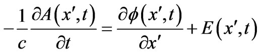
It is therefore clear that finding the appropriate  that achieves the above mapping in full generality will require a careful solution of the system of PDEs (2), applied to only one spatial variable, namely
 (10)
(10)
(with  and
and  ). This system is underdetermined in the sense that we only have knowledge of
  at an initial point
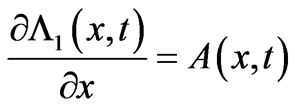
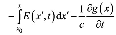
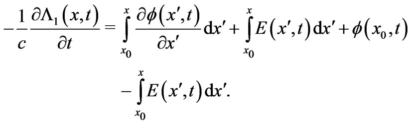
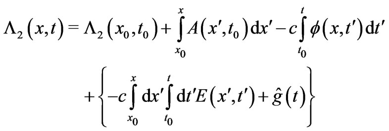
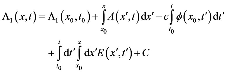
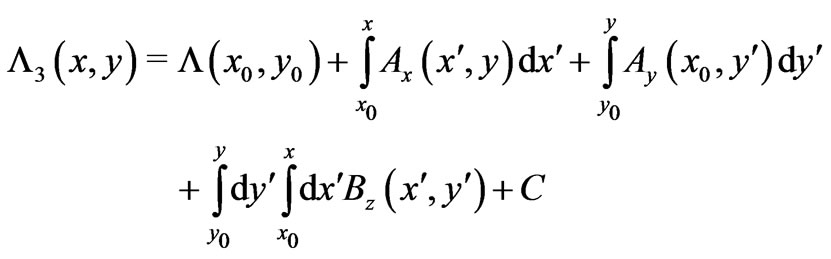
  and with no further boundary conditions (hence multiplicities of solutions being generally expected, see below). By following a careful procedure of integrations [5] we finally obtain 2 distinct solutions (depending on which equation we integrate first): the first solution is
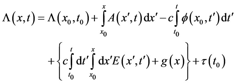 (11)
(11)
with  required to be chosen so that the quantity
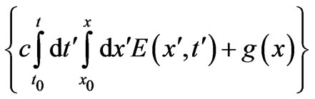 is independent of x, and
(from an inverted route of integrations) the second solution turns out to be
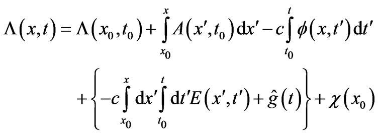 (12)
(12)
with  to be chosen in such a way that
 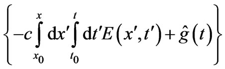 is independent of t.
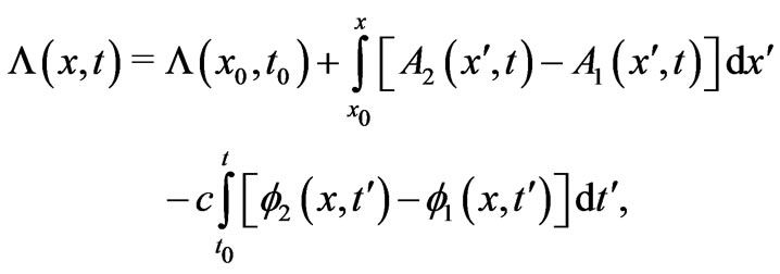
In the above  is the difference of electric fields in the two systems, which can be nonvanishing at regions remote to the observation point
  (see examples later below). (Note again that at the point of observation
 , signifying the basic fact that the fields in the two systems are identical at the observation point
 ). The constant last terms in both solutions can be shown to be related to possible multiplicities of
  (for a full discussion see [5]) and they are zero in simple-connected spacetimes. Also note again that the integrations of potentials in (11) and (12) indeed form paths that continuously connect
  to
to  in the xt-plane (the red-arrow and green-arrow paths of Figure 1(a)), a property that the incorrectly used solution (9) does not have.
By “going backwards” one can directly verify that (11) or (12) are indeed solutions of the basic system of PDEs (10), even for any nonzero  (in regions
 ). Indeed, if we call our first solution (Equation (11)) for simple-connected spacetime
 , namely
 (13)
(13)
with  chosen so that
is independent of x, then we have (even for  for
for ):
):
1)  satisfied trivially
![]() (because the quantity
(because the quantity ![]() is independent of x).
is independent of x).
2) 
 (the last term being trivially zero,
 ), and then with the substitution
we obtain
a) We see that the 2nd and 4th terms of the rhs cancel each other, and b) the 1st term of the rhs is
Hence finally
We have directly shown therefore that the basic system of PDEs (10) is indeed satisfied by our generalized solution  even for any nonzero
  (in regions
 ). (Once again note, however, that at the point of observation
 , indicating the essential fact that the fields in the two systems are equal (recall that
 ) at the observation point
 ). It should be noted that the function
  owes its existence to the fact that the spacetime point of observation
  is outside the E-distribution (hence the term “nonlocal”, used for the effect of the field-difference E on the phases), and the reader can clearly see this in the “striped” E-distributions of the examples that follow later in this Section.
In a completely analogous way, one can easily see that our alternative solution (Equation (12)) also satisfies the basic system of PDEs above. Indeed, if we call our second (alternative) solution (Equation (12)) for simpleconnected spacetime , namely
 (14)
(14)
with  chosen so that
is independent of t, then we have (even for  for
for ):
):
1)  satisfied trivially
 ![]() (because the quantity
(because the quantity ![]() is independent of t).
is independent of t).
2) 
 (the last term being trivially zero,
 ), and then with the substitution
we obtain

a) We see that the 2nd and 4th terms of the rhs cancel each other, and b) the 3rd term of the rhs is
Hence finally

Once again, all the above are true for any nonzero  (in regions
 ) for arbitrary analytical dependence of the remote field-difference on its arguments.
Let us now note that in (11) and (12) the placement of  and
and ![]() gives a “path-sense” to the line integrals in each solution (each path consisting of 2 perpendicular line segments connecting
gives a “path-sense” to the line integrals in each solution (each path consisting of 2 perpendicular line segments connecting  to
to , with solution (11) having a clockwise and solution (12) a counterclockwise sense, see red and green arrow paths in Figure 1); this way a natural rectangle is formed, within which the enclosed “electric fluxes” in spacetime appear to be crucial (showing up as nonlocal contributions of the electric field-differences from regions
  of space and time that are remote to the observation point
 ). These nonlocal terms in
  have a direct effect on the wavefunction-phases at
 . The actual manner in which this happens is determined by the functions
  or
or  -these must be chosen in such a way as to satisfy their respective conditions in (11) and (12). To see how these functions (
 or
or![]() ) are actually determined, and what form the above solutions take in nontrivial cases (and how they give new results, i.e. not differing from the usual ones by a mere constant) let us first take examples of striped E-distributions in spacetime:
) are actually determined, and what form the above solutions take in nontrivial cases (and how they give new results, i.e. not differing from the usual ones by a mere constant) let us first take examples of striped E-distributions in spacetime:
1) For the case of the extended vertical strip (parallel to the t-axis) of Figure 1(a) (the case of a one-dimensional capacitor that is (arbitrarily and variably) charged for all time), then, for x located outside (and on the right of) the capacitor, the quantity  in
in 
is already independent of x (since a displacement of the  -corner of the rectangle to the right, along the x-direction, does not change the enclosed “electric flux”, see Figure 1(a)); hence in this case the function
  can be taken as
  (up to a constant C), because then the condition for
  stated in the solution (11) (namely, that the quantity in brackets must be independent of x) is indeed satisfied. (Note again that the above x-independence of the enclosed “electric flux” is important for the existence of
 ).
).
So for this setup, the nonlocal term in solution  survives (the quantity in brackets is nonvanishing), but it is not constant: this enclosed flux depends on t (since the enclosed flux does change with a displacement of the
  -corner of the rectangle upwards, along the t-direction). Hence, by looking at the alternative solution
 ,
,
 (a)
(a)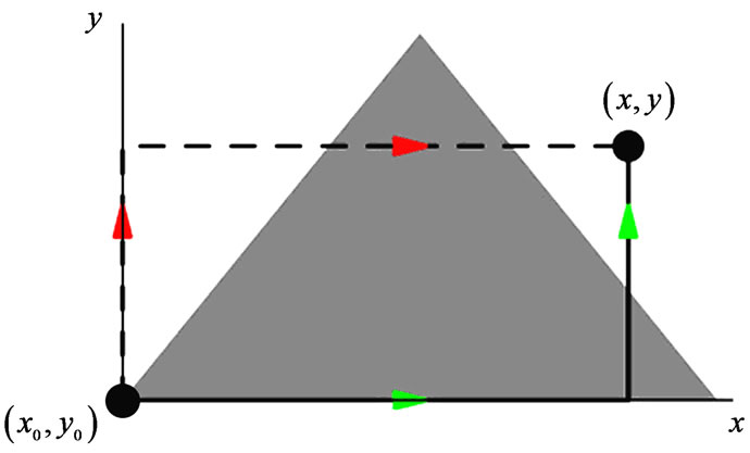 (b)
(b)
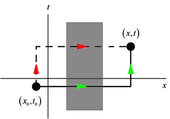
Figure 1. (Color online): Examples of simple field-configuretions (in simple-connected regions), where the nonlocal terms exist and are nontrivial, but can easily be determined: (a) a striped case in 1 + 1 spacetime, where the electric flux enclosed in the “observation rectangle” is dependent on t but independent of x; (b) a triangular distribution in 2-D space, where the part of the magnetic flux inside the corresponding “observation rectangle” depends on both x and y. The appropriate choices for the corresponding nonlocal functions  and
and ![]() for case (a), or
for case (a), or  and
and  for case (b), are given in the text (Sections 3 and 4 respectively).
the quantity  is dependent on t, so that
  must be chosen as
(up to the same constant C) in order to cancel this t-dependence, so that its own condition stated in the solution (12) (namely, that the quantity in brackets must be independent of t) is indeed satisfied; as a result, the quantity in brackets in solution  disappears and there is no nonlocal contribution in
  (for C = 0). (If we had used a
 , the nonlocal contributions would be differently shared between the two solutions, but without changing the Physics when we take the difference of the two solutions, see below).
With these choices of  and
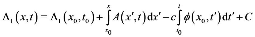
and , we already have new results (compared to the standard ones of the integrals of potentials). i.e. one of the two solutions, namely
  is affected nonlocally by the enclosed flux (and this flux is not constant). Spelled out clearly, the two results are:
 (15)
(15)
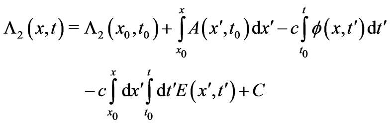
 (16)
(16)
And now it is easy to note that, if we subtract the two solutions  and
and  (and of course assume, as usual, single-valuedness of
  at the initial point
 , i.e.
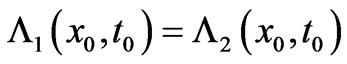 ) the result is zero (i.e. it so happens that the electric flux determined by the potential-integrals is exactly cancelled by the nonlocal term of electric fields (i.e. the term that survives in
  above)), a cancellation effect that is important and that will be generalized in later Sections.
2) In the “dual case” of an extended horizontal strip— parallel to the x-axis (that corresponds to a nonzero electric field in all space that has however a finite duration T), the proper choices (for observation time instant t > T) are basically reverse (i.e. we can now take  and
and
 (since the “electric flux”
enclosed in the “observation rectangle” now depends on x, but not on t), with both choices always up to a common constant) and once again we can easily see, upon subtraction of the two solutions, a similar cancellation effect. In this case again, the results are also new (a nonlocal term survives now in ). Again spelled out clearly, these are:
 (17)
(17)
 (18)
(18)
their difference also being zero.
3) And if we want cases that are more involved (with the nonlocal contributions appearing nontrivially in both solutions  and
and  and with
  and
and  not being “immediately visible”) we must again consider different shapes of E-distribution. One such case (a triangular E-distribution) is shown in Figure 1(b) (for the corresponding magnetic case to be discussed in the next Section, which however is completely analogous); in this case the enclosed flux depends on both x and t (but can be shown to be separable, so that the functions
  and
and  still exist and can easily be found in closed analytical form, see next Section). As for the last constant terms
  and
and  (what we will call “multiplicities”), these are only present (nonvanishing) when
  is expected to be multivalued, i.e. in cases of motion in multiple-connected spacetimes, and are then related to the fluxes in the inaccessible regions: in the electric Aharonov-Bohm setup, the prototype of multiple-connectivity in spacetime [9], it turns out [5] that
 enclosed (and here inaccessible) “electric flux”, and if these values are substituted in (11) and (12) they cancel out the new nonlocal terms and lead to the usual electric Aharonov-Bohm result (of mere integrals over potentials). As for other, more esoteric properties of the new solutions in simple-connected spacetimes, it can be rigorously shown [5] that solutions (11) and (12) are actually equal, because
  turns out to be equal to the t-independent bracket of (12), and
  turns out to be equal to the x-independent bracket of (11), the nonlocal terms having therefore the tendency to exactly cancel the “Aharonov-Bohm terms” (this being true for arbitrary shapes and analytical form of
 ).
).
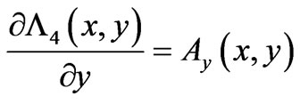
4. 2-D Static Case
After having discussed fully the simple  -case, let us for completeness give the analogous (Euclidian-rotated in 4-D spacetime) derivation for
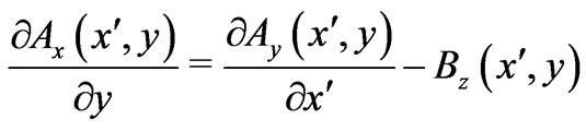
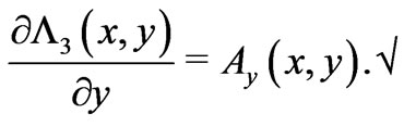
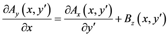
  -variables and briefly discuss the properties of the simpler static solutions in spatial two-dimensionality. We will simply need to apply the same methodology (of solution of a system of PDEs) to such static spatially two-dimensional cases (so that now different (remote) magnetic fields for the two systems, perpendicular to the 2-D space, will arise). For such cases we need to solve the system of PDEs that is now of the form
 (19)
(19)
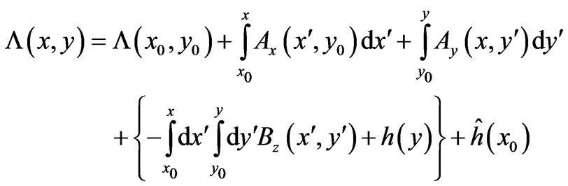
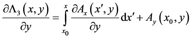
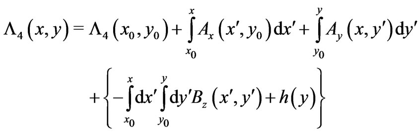
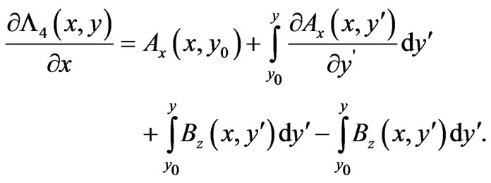
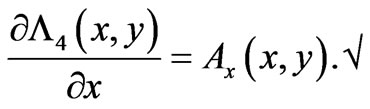
By following then a similar procedure of integrations [5] we obtain the following general solution
 (20)
(20)
with  chosen so that
 :
:
is independent of x, a result that applies to cases where the particle goes through different perpendicular magnetic fields  and
and  in spatial regions that are remote to (i.e. do not contain) the observation point
  (and in the above
 ). The reader should note that the first 3 terms of (20) are the (total) Dirac phase along two perpendicular segments that continuously connect the initial point
  to the point of observation
 , in a clockwise sense (see for example the red-arrow paths in Figure 1(b)). But apart from this Dirac phase, we also have nonlocal contributions from
  and its flux within the “observation rectangle” (see i.e. the rectangle being formed by the redand green-arrow paths in Figure 1(b))). Below we will directly verify that (20) is indeed a solution of (19) (even for
  for
for ). Alternatively, by following the reverse route of integrations, we finally obtain the following alternative general solution
 (21)
(21)
with  chosen so that
 : is independent of y, and again the reader should note that, apart from the first 3 terms (the (total) Dirac phase along the two other (alternative) perpendicular segments (connecting
  to
to ), now in a counterclockwise sense (the green-arrow paths in Figure 1(b))), we also have nonlocal contributions from the flux of
  that is enclosed within the same “observation rectangle” (that is naturally defined by the four segments of the two solutions (Figure 1(b)).
In all the above,  and
and  are the Cartesian components of
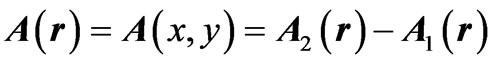 , and, as already mentioned,
  is the difference between (perpendicular) magnetic fields that the two systems may experience in regions that do not contain the observation point
  i.e.
i.e.
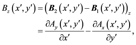
and, although at the point of observation  we have
  (already emphasized in the Introductory Sections), this
  can be nonzero for
 . It should be noted that it is because of
  that the functions
  and
and  of (20) and (21) can be found, and the new solutions therefore exist (and are nontrivial). For the impatient reader, simple physical examples with the associated analytical forms of
  and
and  (derived in detail) are given later in this Section.
One can again show that the 2 solutions are equal for simple-connected space (when the last constant terms  and
and  are vanishing), and for multipleconnectivity the values of the multiplicities
  and
and  cancel out the nonlocalities and reduce the above to the usual result of mere A-integrals along the 2 paths (i.e. two simple Dirac phases).
A direct “backwards” verification that (20) and (21) do indeed satisfy the basic system (19) (even for cases with  in remote regions of space) can be made along similar lines to the ones of the last Section: for simple-connected space, let us call our solution (20)
 , namely
 (22)
(22)
with  chosen so that
  is independent of x. We then have (even for
  for
for ):
):
1)  satisfied trivially
  (because the quantity
 ![]() is independent of x).
is independent of x).
2) 

(the last term being trivially zero, ), and then with the substitution
we obtain

a) We see that the 2nd and 4th terms of the right-handside (rhs) cancel each other, and b) the 1st term of the rhs is

Hence finally
We have directly shown therefore (by “going backwards”) that the basic system of PDEs (19) is indeed satisfied by our generalized solution  even for any nonzero
  (in regions
 ; recall that always
 ). To fully appreciate the above simple proof, the reader is again urged to look at the cases of “striped”
  -distributions later below, the point of observation
  always lying outside the strips, so that the above function
  can easily be determined, and the new solutions really exist—and they are nontrivial.
In a completely analogous way, one can easily see that our alternative solution (Equation (21)) also satisfies the basic system of PDEs above. Indeed, if we call this second static solution , namely
 (23)
(23)
with ![]() chosen so that
chosen so that  is independent of y, then we have (even for
  for
for ):
):
1)  satisfied trivially
 ![]() (because the quantity
(because the quantity ![]() is independent of y).
is independent of y).
2) 

(the last term being trivially zero, ), and then with the substitution
we obtain
a) We see that the last two terms of the rhs cancel each other, and b) the 2nd term of the rhs is

Hence finally
Once again, all the above are true for any nonzero  (in regions
 ) for arbitrary analytical dependence of the remote field-difference on its arguments. And for a clearer understanding of this proof let us now turn to the “striped” examples promised earlier.
In order to see again how the above solutions appear in nontrivial cases (and how they give completely new results, i.e. not differing from the usual ones (i.e. from the Dirac phase) by a mere constant) let us first take examples of striped  -distributions in space:
1) For the case of an extended vertical strip—parallel to the y-axis, such as in Figure 1(a) (imagine t replaced by y) (i.e. for the case that the particle has actually passed through nonzero , hence through different magnetic fields in the two (mapped) systems), then, for x located outside (and on the right of) the strip, the quantity
  in
in  is already independent of x (since a displacement of the
  -corner of the rectangle to the right, along the x-direction, does not change the enclosed magnetic flux—see Figure 1(a) for the analogous
  -case discussed earlier). Indeed, in this case the above quantity (the enclosed flux within the “observation rectangle”) does not depend on the x-position of the observation point, but on the positioning of the boundaries of the
  -distribution in the x-direction (better, on the constant width of the strip)—as the x-integral does not give any further contribution when the dummy variable
  goes out of the strip. In fact, in this case the enclosed flux depends on y as we discuss below (but, again, not on x). Hence, for this case, the function
  can be easily determined: it can be taken as
  (up to a constant C), because then the condition for
  stated in solution (20) (namely, that the quantity in brackets must be independent of x) is indeed satisfied.
We see therefore above that for this setup, the nonlocal term in solution  survives (the quantity in brackets is nonvanishing), but it is not constant: as already noted, this enclosed flux depends on y (since the enclosed flux does change with a displacement of the
  -corner of the rectangle upwards, along the y-direction, as the y-integral is affected by the positioning of y—the higher the positioning of the observation point the more flux is enclosed inside the observation rectangle). Hence, by looking at the alternative solution
  the quantity
  is dependent on y, so that
  must be chosen as
  (up to the same constant C) in order to cancel this y-dependence, so that its own condition stated in solution (21) (namely, that the quantity in brackets must be independent of y) is indeed satisfied; as a result, the quantity in brackets in solution
  disappears and there is no nonlocal contribution in
  (for
(for ). (If we had used a
 , the nonlocal contributions would be shared between the two solutions in a different manner, but without changing the Physics when we take the difference of the two solutions (see below)). [The crucial point in the above for the existence of
  and
and  is, once again, the fact that
  at
at , combined with the sharp boundaries of the nonvanishing
  -region].
With these choices of  and
and , we already have new results (compared to the standard ones of the integrals of potentials). i.e. one of the two solutions, namely
  is affected nonlocally by the enclosed flux (and this flux is not constant). Spelled out clearly, the two results are:
 (24)
(24)
 (25)
(25)
And now it is easy to note that, if we subtract the two solutions  and
and , the result is zero (because the line integrals of the vector potential A in the two solutions are in opposite senses in the
  plane, hence their difference leads to a closed line integral of A, which is in turn equal to the enclosed magnetic flux, and this flux always happens to be of opposite sign from that of the enclosed flux that explicitly appears as a nonlocal contribution of the
  -fields (i.e. the term that survives in
  above). Hence, the two solutions are equal. [We of course everywhere assumed, as usual, single-valuedness of
  at the initial point
 , i.e.
 matters of multivaluedness of
  at the observation point
  will be addressed later below].
It is interesting that, formally speaking, the above equality of the two solutions is due to the fact that the x-independent quantity in brackets of the 1st solution (20) is equal to the function  of the 2nd solution (21), and the y-independent quantity in brackets of the 2nd solution (21) is equal to the function
  of the first solution (20). This turns out to be a general behavioral pattern of the two solutions in simple-connected space, that is valid for any shape (and any analytical form) of
  -distribution. But most importantly, it should be noted that this vanishing of
  is a cancellation effect that is emphasized further later below and discussed in completely physical terms.
2) In the “dual case” of an extended horizontal strip— parallel to the x-axis, the proper choices (for y above the strip) are basically reverse (i.e. we can now take 
and 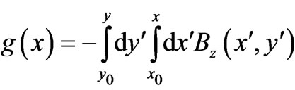 (since the flux enclosed in the rectangle now depends on x, but not on y), with both choices always up to a common constant) and once again we can easily see, upon subtraction of the two solutions, a similar cancellation effect. In this case as well, the results are again new (a nonlocal term survives now in
 ). Again spelled out clearly, these are:
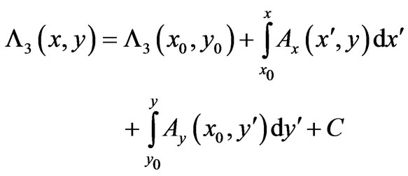 (26)
(26)
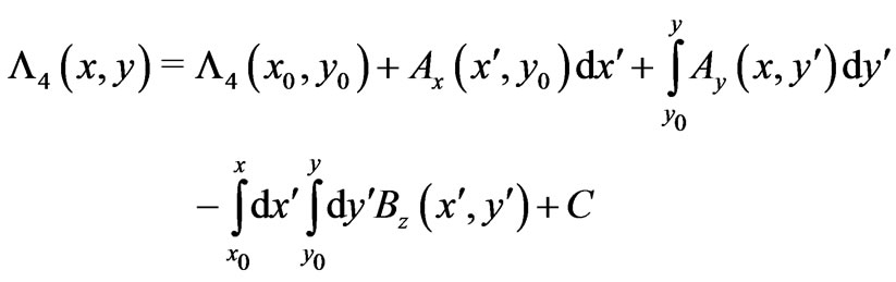 (27)
(27)
(their difference also being zero). Again here the crucial point is that, because the  -configuration does not contain the point
 , a displacement of this observation point upwards does not change the flux inside the “observation rectangle”; this makes the new solutions (i.e. the functions
  and
and ) exist.
3) And if we want cases that are more involved (i.e. with the nonlocal contributions appearing nontrivially in both solutions  and
and  and with
  and
and  not being “immediately visible”), we must consider different shapes of
  -distributions. One such case is a triangular one that is shown in Figure 1(b) (for simplicity an equilateral triangle, and with the initial point
 ) and with the point of observation
  being fairly close to the triangle’s right side as in the figure. Note that for such a configuration, the part of the magnetic flux that is inside the “observation rectangle” (defined by the right upper corner
 ) depends on both x and y. It turns out, however, that this (x and y)— dependent enclosed flux can be written as a sum of separate xand y-contributions, so that appropriate
  and
and  can still be found (each one of them must be chosen so that it only cancels the corresponding variable’s dependence of the enclosed flux). For a homogeneous
  it is a rather straightforward exercise to determine this enclosed part, i.e. the common area between the observation rectangle and the equilateral triangle, and from this we can find the appropriate
  that will cancel the x-dependence, and the appropriate
  that will cancel the y-dependence. These appropriate choices turn out to be
 (28)
(28)
and
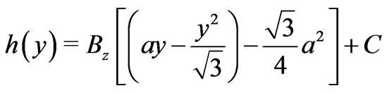 (29)
(29)
with a being the side of the equilateral triangle. We should emphasize that expressions (28) and (29), if combined with (20) or (21), give the nontrivial nonlocal contributions of the field-difference  of the remote magnetic fields on
  of each solution (hence on the phase of the wavefunction of each wavepacket travelling along each path) at the observation point
 , that always lies outside the
  -triangle. (We mention again that in the case of completely spread-out states, the equality of the two solutions at the observation point essentially demonstrates the uniqueness (single-valuedness) of the phase in simple-connected space). Further physical discussion of the above cancellations, and a semiclassical interpretation, is given later below.
Finally, in more “difficult” geometries, i.e. when the shape of the  -distribution is such that the enclosed flux does not decouple in a sum of separate xand ycontributions, such as cases of circularly shaped
  - distributions, it is advantageous to solve the system (19) directly in non-Cartesian (i.e. polar) coordinates [5]. A general comment that can be made for general shapes is that, depending on the geometry of shape of the
  - distribution, an appropriate change of variables (to a new coordinate system) may first be needed, so that generalized solutions of the system (19) can be found (namely, so that the enclosed flux inside the transformed observation rectangle (i.e. a slice of an annular section in the case of polar coordinates) can be written as a sum of separate (transformed) variables), and then the same methodology (as in the above Cartesian cases) can be followed.
As we saw in the above examples, in case of a stripeddistribution of the magnetic field difference , the functions
  and
and  in (20) and (21) have to be chosen in ways that are compatible with their corresponding constraints (stated after (20) and (21)). By then taking the difference of (20) and (21)) we obtain that the “Aharonov-Bohm phase” (the one originating from the closed line integral of A’s) is exactly cancelled by the additional nonlocal term of the magnetic fields (that the particle passed through). This is quite reminiscent of the cancellation of phases observed in the early experiments of Werner & Brill [10] for particles passing through a magnetic field (a cancellation between the “AharonovBohm phase” and the semiclassical phase picked up by the trajectories), and our method seems to provide a natural explanation: as our results are general (and for delocalized states in simple-connected space they basically demonstrate the uniqueness of
 ), they are also valid and applicable to states that describe wavepackets in classical motion, as was the case of the Werner & Brill experiments. (A similar cancellation of an electric Aharonov-Bohm phase, that has never been noted in the literature, also occurs for particles passing through a static electric field, and this we will independently prove below, again for semiclassical states). We conclude that, for static cases, and when particles pass through nonvanishing classical fields, the new nonlocal terms reported in the present work lead quite generally to a cancellation of Aharonov-Bohm phases that had earlier been only sketchily noticed and only at the semiclassical (magnetic) level.
What is however more important to point out here is that the above cancellations can be understood as a compatibility between the Aharonov-Bohm fringe-displacement and the trajectory-deflection due to the Lorentz force (i.e. the semiclassical phase picked up due to the optical path difference of the two deflected trajectories exactly cancels (is opposite in sign from) the “AharonovBohm phase” picked up by the same trajectories due to the flux that they enclose). This opposite sign seems to have been rather unnoticed: In Feynman’s Figure 15-8 [11], or in Felsager’s Figure 2.16 [12], the classical trajectories are deflected after passing through a strip of a magnetic field placed on the right of a double-slit apparatus. Both authors determine the semiclassical phase picked up by the deflected trajectories and find it consistent with the Aharonov-Bohm phase. One can see on closer inspection, however, that the two phases actually have opposite signs (see our own Figure 2 and the discussion that follows below, where this is proved in detail). Similarly, in the very recent review of Batelaan & Tonomura [13], their Figure 2 shows wavefronts associated to the deflected classical trajectories where it is stated that “the phase shift calculated in terms of the Lorentz force is the same as that predicted by the Aharonov-Bohm effect in terms of the vector potential”. Once more, however, it turns out that the sign of the classical phase-difference is really opposite to the sign of the Aharonov-Bohm phase (see proof below). The phases are not equal as stated by the authors. And it turns out that even “electric analogs” of the above cases also demonstrate this opposite-sign relationship (see proof further below). All the above examples can be viewed as a manifestation of the cancellations that have been found in the present work for general (even completely spreadout) quantum states (but in these examples they are just special cases for narrow wavepacket-states in classical motion).
Let us give a brief elementary proof of the above claimed opposite sign-relationships: Indeed, in our Figure 2, the “Aharonov-Bohm phase” due to the flux enclosed between the two classical trajectories (of a particle of charge q) is
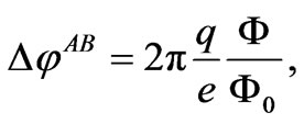 (30)
(30)
with  the flux quantum, and
  the enclosed flux between the two trajectories (for small trajectory-deflections), with the deflection originating from the presence of the magnetic strip B and the associated Lorentz forces. On the other hand, the semiclassical phase difference between the same 2 classical trajectories is
 , with
  being the de Broglie wavelength (and v being the speed of the particle, taken almost constant (as usually done) due to the small deflections), and with
  being
being 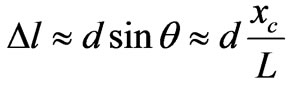 (
(
being the (displaced) position of the central fringe on the screen). We have therefore
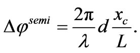 (31)
(31)
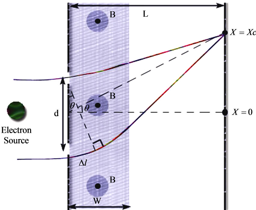
Figure 2. (Color online): The standard double-slit apparatus with an additional strip of a perpendicular magnetic field B of width W placed between the slit-region and the observation screen. In the text we deal for simplicity with the case  so that deflections (of the semiclassical trajectories) due to the Lorentz force, shown here for a negative charge q, are very small.
Now, the Lorentz force (exerted only during the passage through the thin magnetic strip, hence only during a time interval ) has a component parallel to the screen (let us call it x-component) that is given by
 (32)
(32)
which shows that there is a change of kinematic momentum (parallel to the screen) equal to  or, equivalently, a change of parallel speed
 (33)
(33)
which is the speed of the central fringe’s motion (i.e. its displacement over time along the screen). Although this has been caused by the presence of the thin deflecting magnetic strip, this displacement is occuring uniformly during a time interval  and this time interval must satisfy
 (34)
(34)
(as, for small displacements, the wavepackets travel most of the time in uniform motion, i.e. ). We therefore have that the central fringe displacement must be
 and noting that
 , we finally have
 (35)
(35)
By susbstituting (35) into (31), the lengths L and ![]()
cancel out, and we finally have  which with
  the flux quantum, and
the enclosed flux (always for small trajectory-deflections) gives (through comparison with (30)) our final proof that
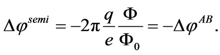 (36)
(36)
[It should be noted that such an opposite sign relation actually tells us that the total (semiclassical + AB) phase difference is zero at the new position of the central (bright) fringe (after it has been displaced due to the trajectories’ deflection), and in this sense the above minus sign should be rather expected.]
The “electric analog” of the above exercise is also outlined below, now with a homogeneous electric field (pointing downwards everywhere in space, but switched on for only a finite duration T) on the right of a doubleslit apparatus (see our Figure 3): In this case the electric Lorentz force qE is exerted on the trajectories only during the small time interval  which we take to be much shorter (
 ) than the time of travel
  (we now have a thin electric strip in time rather than the thin magnetic strip in space that we had earlier). The electric type of “Aharonov-Bohm phase” is now
 (37)
(37)
with  being the electric potential difference between the two trajectories, hence
  (again for small trajectory-deflections). On the other hand, the semiclassical phase difference between the two trajectories is again given by (31), but the position
  of the central fringe must now be determined by the electric field force qE: The change of kinematic momentum (always parallel to the screen) is now qET, hence the analog of (33) is now
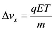 (38)
(38)
which if combined with (34) (that is obviously valid in this case as well, again for small deflections, due to the
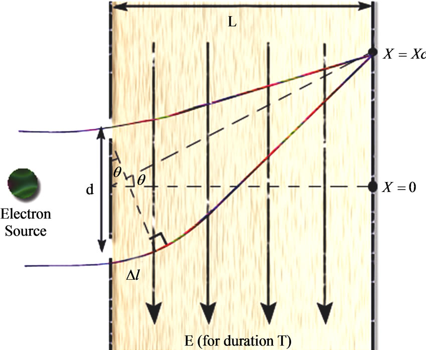
Figure 3. (Color online): The analog of Figure 2 (again for a negative q) but with an additional electric field parallel to the observation screen that is turned on for a time interval T. In the text we deal for simplicity with the case  (with
(with ,
,  the de Broglie wavelength), so that deflections (of the semiclassical trajectories) due to the electric force are again very small. For both Figures 2 and 3, it is shown in the text that
 , hence we observe an extra minus sign compared to what is usually reported in the literature.
 ), and always with
 , gives that the central fringe displacement must be
 , and using again
 , we finally have the following analog of (35)
 (39)
(39)
By substituting (39) into (31), the lengths L and ![]() again cancel out, and we finally have
again cancel out, and we finally have
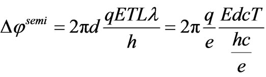 , which with
the flux quantum, and through comparison with (37) leads once again to our final proof that
 (40)
(40)
We note therefore that even in the electric case, the semiclassical phase difference (between two trajectories) picked up due to the Lorentz force (exerted on them) is once again opposite to the electric “Aharonov-Bohm phase” picked up by the same trajectories (due to the electric flux that they enclose).
We should point out once again, however, that although the above elementary considerations apply to semiclassical motion of narrow wavepackets, in this paper we have given a more general understanding of the above opposite sign-relationships that applies to general (even completely delocalized) states, and that originates from what could be called “ generalized Werner & Brill cancellations” (the cancellations that come out of our new solutions, in cases more general than those of Werner & Brill, including both magnetic and electric fields, both static and t-dependent situations, and both semiclassical and spread-out quantum states).
In a slightly different vein, the cancellations that we found above give an explanation of why certain classical arguments (invoking the past t-dependent history of an experimental setup) seem to be successful in giving at the end an explanation of Aharonov-Bohm effects (namely a phase consistent with that of a static Aharonov-Bohm configuration). However, there is again an opposite sign that seems to have been largely unnoticed in such arguments as well (i.e. in Silverman [14], where in his Equation (1.34) there should be an extra minus sign). Our above observation essentially describes the fact that, if we had actually used a t-dependent magnetic flux (with its final value being the actual value of our static flux), then the induced electric field (viewed now as a nonlocal term of the present work) would have cancelled the static Aharonov-Bohm phase. Of course now, this t-dependent experimental set up has not been used (the flux is static) and we obtain the usual magnetic Aharonov-Bohm phase, but the above argument (of a “potential experiment” that could have been carried out) takes the “mystery” away of why such history-based arguments generally work— although they have to be corrected with a sign. The above also gives a rather natural account of the “dynamical nonlocality” character [2] attributed to the various Aharonov-Bohm phenomena (magnetic, electric or combined), although—in the present work—this dynamical quantum nonlocality seems to simultaneously respect Causality, as will be seen in the next Section. This is a rather pleasing characteristic of this theory that, as far as we are aware, has no parallel in other formulations.
5. Full (x,y,t)-Case
Finally, let us look at the most general spatially-twodimensional and time-dependent case. This combines effects of (perpendicular) magnetic fields (which, if present only in physically-inaccessible regions, can have Aharonov-Bohm consequences) with the temporal nonlocalities of electric fields (parallel to the plane) found in previous Sections. By working again in Cartesian spatial coordinates, we now have to deal with the full system of PDEs
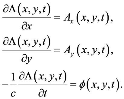 (41)
(41)
This exercise is considerably longer than the previous ones but important to solve, in order to see in what manner the solutions of this system are able to combine the spatial and temporal nonlocal effects found above. There are now 3! = 6 alternative integration routes to follow for solving this system (and, in addition to this, the results in intermediate steps tend to proliferate). The corresponding (rather long) procedure for solving the system (41) is described in detail in [5], and 2 out of the 12 solutions that can be derived turn out to be the most crucial for the discussion that will follow. First, by following steps similar to the ones of Section 4, the following temporal generalization of (21) is obtained
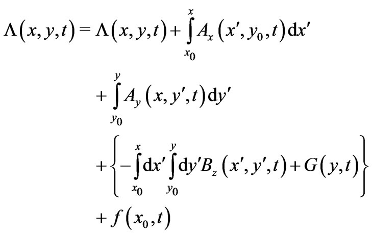 (42)
(42)
with  such that
 is independent of yand from this point on, the third equation of the system (41) is getting involved to determine the nontrivial effect of scalar potentials on
  Indeed, by combining it with (42) there results a wealth of patterns, one of them leading finally to our first solution, namely
 (43)
(43)
with the functions  and
and  to be chosen in such a way as to satisfy the following 3 independent conditions:
 (44)
(44)
which is of course a special case of the condition on  above (see after (42)) applied at
 , and the other 2 turn out to be of the form
 (45)
(45)
 (46)
(46)
(It is probably important to note that for the above results the Faraday’s law is crucial [5]). As for the constant quantity  appearing in (43), it again describes possible effects of multiple-connectivity at the instant
 ![]() (which are absent for simple-connected spacetimes, but will be crucial in the discussion of the van Kampen thought-experiment to be discussed later below).
(which are absent for simple-connected spacetimes, but will be crucial in the discussion of the van Kampen thought-experiment to be discussed later below).
Equation (43) is our first solution. It is now crucial to note that an alternative form of solution (with the functions G and F satisfying the same conditions as above) can be derived, and it turns out to be
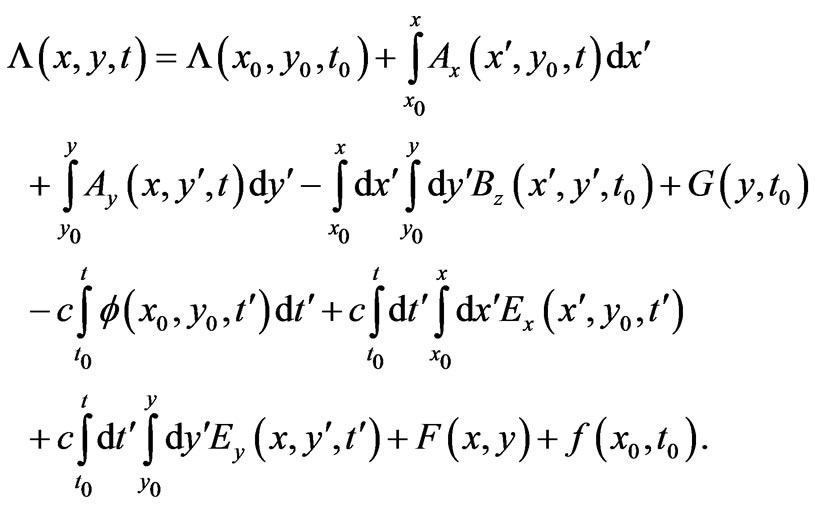 (47)
(47)
In this alternative solution we note that, in comparison with (43), the line-integrals of E have changed to the other alternative “path” (note the difference in the placement of the coordinates of the initial point  in the arguments of
  and
and  compared to (43)) and they happen to have the same sense as the A-integrals, while simultaneously the magnetic flux difference shows up with its value at the initial time
 ![]() rather than at t. This alternative form will be shown to be useful in cases where we want to directly compare physical situations in the present (at time t) and in the past (at time
rather than at t. This alternative form will be shown to be useful in cases where we want to directly compare physical situations in the present (at time t) and in the past (at time![]() ), and the above noted change of sense of E-integrals (compared to (43)) will be crucial in the discussion that follows below. (It is also important here to note that, in the form (47), the electric fields have already incorporated the effect of radiated
), and the above noted change of sense of E-integrals (compared to (43)) will be crucial in the discussion that follows below. (It is also important here to note that, in the form (47), the electric fields have already incorporated the effect of radiated  -fields in space (through the Maxwell’s equations, see [5]), and this is why at the end only the
  at
at ![]() appears explicitly).
appears explicitly).
Once again the reader can directly verify that (43) or (47) indeed satisfy the basic input system (41). (This verification is considerably more tedious than the earlier ones but rather straightforward).
But a last mathematical step remains: in order to discuss the van Kampen case, namely an enclosed (and physically inaccessible) magnetic flux (which however is time-dependent), it is important to have the analogous forms through a reverse route of integrations (see [5]), where at the end we will have the reverse “path” of A-integrals (so that by taking the difference of the resulting solution and the above solution (43) (or (47)) will lead to the closed line integral of A, which will then be immediately related to van Kampen’s magnetic flux (at the instant t)). By following then the reverse route, and by applying a similar strategy at every intermediate step, we finally obtain the following solution (the spatially “dual” of (43)), namely
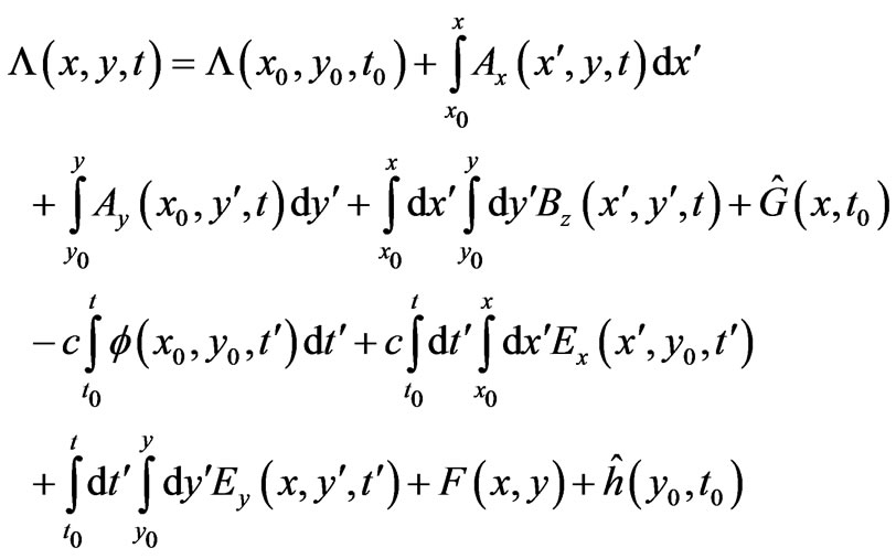 (48)
(48)
with the functions  and
and  to be chosen in such a way as to satisfy the following 3 independent conditions:
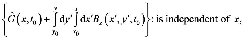 (49)
(49)
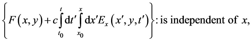 (50)
(50)
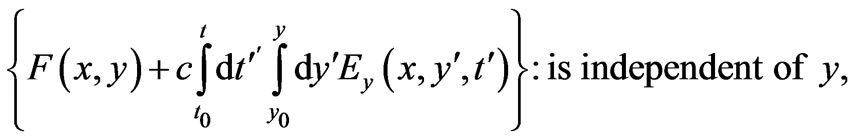 (51)
(51)
where again for the above results the Faraday’s law is crucial. The corresponding analog of the alternative form (47) (where  appears at
![]() ) is more important for the discussion that follows and turns out to be
) is more important for the discussion that follows and turns out to be
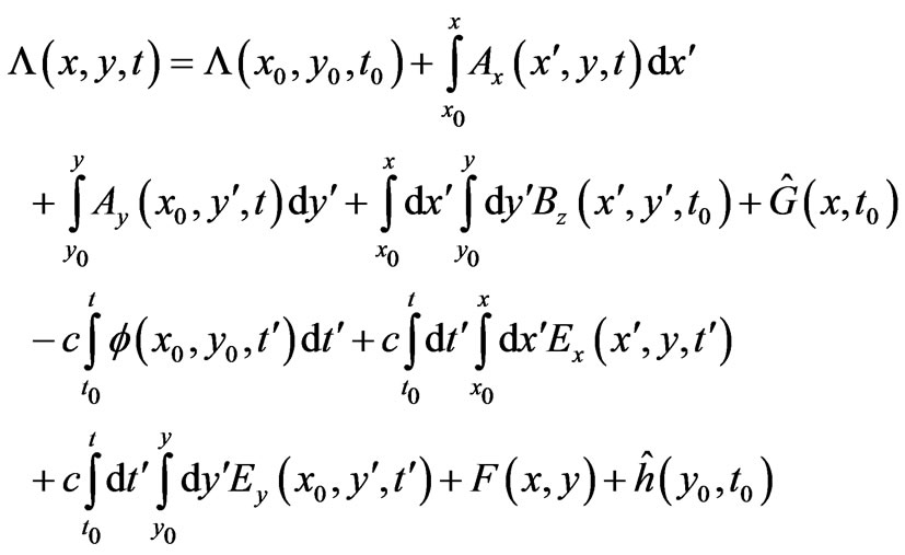 (52)
(52)
with  and
and  following the same 3 conditions above. The constant term
  again describes possible multiplicities at the instant
![]() ; it is absent for simple-connected spacetimes, but will be crucial in the discussion of the van Kampen thought-experiment.
; it is absent for simple-connected spacetimes, but will be crucial in the discussion of the van Kampen thought-experiment.
In (48) (and in (52)), note the “alternative paths” (compared to solution (43) (and (47))) of line integrals of A’s (or of E’s). But the most crucial element for what follows is the need to exclusively use the forms (47) and (52) (where  only appears at
![]() ), and the fact that, within each solution, the sense of A-integrals is the same as the sense of the E-integrals. (This is not true in the other solutions where
), and the fact that, within each solution, the sense of A-integrals is the same as the sense of the E-integrals. (This is not true in the other solutions where  appears, as the reader can directly see). These facts will be crucial to the discussion that follows, which briefly addresses the so called “van Kampen paradox”.
In [15] van Kampen considered a magnetic AharonovBohm setup, but with an inaccessible magnetic flux that is t-dependent: he envisaged turning on the flux very late, or equivalently, observing the interference of the two wavepackets on a distant screen very early, earlier than the time it takes light to travel the distance to the screen
(i.e. ), hence using the (instantaneous nature of the)
Aharonov-Bohm phase to transmit information (on the presence of a confined flux somewhere in space) superluminally. Indeed, the Aharonov-Bohm phase at any t is determined by differences of  with
with 
 (basically a special case of (5)). Howeverif we use, instead, our results (47) and (52) above (that contain the additional nonlocal terms), it turns out that, for a spatially-confined magnetic flux
 , the functions G,
  and F in the above solutions can then all be taken zero: 1) their conditions are all satisfied for a flux
  that is not spatially-extended (hence, from the 2 conditions on G and
  (Equation (44) and (49)) we obtain
  since the integrals in brackets are all independent of x and y), and 2) for
 , the integrals of
  and
and  in the corresponding conditions (Equation (45) and (46)) are already independent of both x and y (since
  for all
 with
with  the observation point [the essential point being that at instant t, the E-field has not yet reached the spatial point
  of the screen, and therefore all integrations of
  and
and  with respect to
  and
and  will be contributing only up to a light-cone (see Figure 4) and they will therefore give results that are independent of the integration upper limits x and ybasically a generalization of the striped cases that we saw earlier but now to the case of 3 spatio-temporal variables (with now the spatial point
  being outside the light-cone defined by t (see Figure 4; in this figure the initial spatial point
 , taken for simplicity at
 , has been supposed to be in the area of the inaccessible flux
 , so that, for
 , we have indeed that
 , as written on the figure))]; we therefore rigorously obtain
 ). Moreover, the Aharonov-Bohm multiplicities (at
![]() ) lead to cancellation of the
) lead to cancellation of the  -terms (always at
![]() ), with the final result (after subtraction of the 2 solutions) being
), with the final result (after subtraction of the 2 solutions) being
 (53)
(53)
This can equivalently be written as
 (54)
(54)
which, with  the instantaneous enclosed magnetic flux and with the help of Faraday’s law
  gives
gives
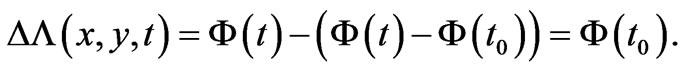 (55)
(55)
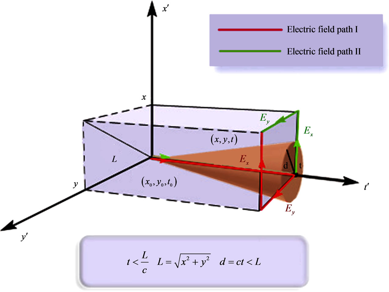
Figure 4. (Color online): The analog of paths of Figure 1 but now in 2 + 1 spacetime for the van Kampen thought-experiment, when the instant of observation t is so short that the physical information has not yet reached the spatial point of observation (x, y). The two solutions (that, for wavepackets, have to be subtracted in order to give the phase difference at (x, y, t)) are given in the text, and are here characterized through their electric field E-line integral behavior: “electric field path (I)” (the red-arrow route) denotes solution (52), and “electric field path (II)” (the green-arrow route) denotes solution (47). Note that the strips of Figure 1(a) have now given their place to a light-cone. At the point of observation (that lies outside this light-cone) the Aharonov-Bohm phase difference has now become “causal” due to cancellations between the two solutions (the two “electric field paths” above).
Although  is generally t-dependent, we obtain the intuitive (causal) result that, for
  (i.e. if the physical information has not yet reached the screen), the phase-difference turns out to be t-independent, and leads to the magnetic Aharonov-Bohm phase that we would observe at
![]() . The new nonlocal terms have conspired in such a way as to exactly cancel the Causality-violating Aharonov-Bohm phase (that would be proportional to the instantaneous
. The new nonlocal terms have conspired in such a way as to exactly cancel the Causality-violating Aharonov-Bohm phase (that would be proportional to the instantaneous ). This gives an honest resolution of the van Kampen “paradox” within a canonical formulation, without using any vague electric Aharonov-Bohm argument (as there is no multiple-connectivity in the
  -plane [9]). An additional physical element is that, for the above cancellation, it is not only the E-fields but also the t-propagation of the
  -fields (the full “radiation field”) that plays a role [5].
Use of other 10 solutions that rigorously come out from the basic system of PDEs can also address boundstate analogs (i.e. in t-dependent magnetic flux-driven 1-D nanorings, such as in [16]) or even “electric” analogs of the above van Kampen case: In Peshkin’s review [3] on the electric Aharonov-Bohm effect, the author correctly states “One cannot wait for the electron to pass and only later switch on the field to cause a physical effect”. Although Peshkin uses his Equation (B.5) and (B.6) (based on the incorrect (5)), he carefully states that it is not the full solution; actually, if we view it as an ansatz, then it is understandable why he needs to enforce a condition (his Equation (B.8), and later (B.9)) on the electric field outside the cages (in order for certain (annoying) terms (resulting from a minimal substitution due to the incorrect ansatz) to vanish and for (B.5) to be a solution). But then he notes that the extra condition cannot always be satisfied (hence (B.5) is not really the solution for all times), drawing from this the above qualitatively correct conclusion on Causality. As it turns out, our treatment gives exactly what Peshkin describes in words (with the total “radiation field” outside the cages being once again crucial in recovering Causality), in a similar way as in the case presented above in this Section for the usual (magnetic) version of the van Kampen experiment. In this “electric analog” that we are discussing now, the causally-offending part of the electric Aharonov-Bohm phase difference will be cancelled by a magnetic type of phase, that originates from the magnetic field that is associated with the t-dependence of the electric field E outside the cages. We conclude that our (exact) results accomplish precisely what Peshkin has in mind in his discussion (on Causality), but in a direct and fully quantitative manner, and with no ansatz based on an incorrect form.
6. Discussion
Returning for the moment to only one of the many misconceptions briefly pointed out in this paper, we should emphasize further that improper uses of simple Dirac phases in the literature are not rare or marginal: even in Feynman [11] it is stated that the simple phase factor  is valid even for dynamic fields; this is also explicitly stated in Erlichson’s review [17]—Silverman [14] being the only report that we are aware of with a careful wording about (5) being only restrictedly valid (for t-independent A and r-independent
 ), although even there the nonlocal terms have been missed.
With respect to the presence of fields in the phases of quantum mechanical wavefunctions that we find, it should be stressed that at the level of the basic Lagrangian  there are no fields present, and the view holds in the literature [18] that electric fields or magnetic fields cannot contribute directly to the phase. This view originates from the pathintegral treatments widely used (where the Lagrangian determines directly the phases of Propagators), but, nevertheless, our canonical treatment shows that fields do contribute nonlocally, and they are actually crucial in recovering Relativistic Causality. Moreover, path-integral discussions [19] of the van Kampen case use wave (retarded)-solutions for A (hence in the Lorenz gauge) and are incomplete; our results take advantage of the retardation of fields E and B (true in any gauge), and not of potentials. In addition, Troudet [19] correctly states that his path-integral treatment is good for not highlydelocalized states in space, and that in case of delocalization the proper treatment “would be much more complicated, and would require a much more complete analysis”. It is fair to state that such a complete analysis has actually been provided in the present work. It should be added that the van Kampen “paradox” seems to be still thought of as “remarkable” [20]. The present work has provided a natural and general resolution, and most importantly, through nonlocal (and Relativistically causal) propagation of wavefunction-phases.
Finally, in trying to explore an even broader significance of the new solutions, one may wonder about possible consequences of the nonlocal terms if these are included in more general physical models that have a gauge structure (in Condensed Matter or High Energy Physics). It is also worth mentioning that if one follows the same “unconventional” method (of solution of PDEs) with the Maxwell’s equations for the electric and magnetic fields (rather than with the PDEs of Equation (2) for the potentials that give ), the corresponding nonlocal terms can be derived in a similar manner, and one can then see that these nonlocal terms essentially demonstrate the causal propagation of the radiation electric and magnetic fields outside physically inaccessible confined sources (i.e. solenoids or electric cages). Although this is of course widely known at the level of classical fields, a major conclusion that can be drawn from the present work (at the level of gauge transformations) is that a corresponding Causality also exists at the level of quantum mechanical phases as well, and this is enforced by the nonlocal terms in t-dependent cases. It strongly indicates that the nonlocal terms found in this work at the level of quantum mechanical phases reflect a causal propagation of wavefunction phases in the Schrödinger Picture (at least one part of them—the one containing the fields—which competes with the Aharonov-Bohm types of phases containing the potentials). This is an entirely new concept (given the local nature but also the nonrelativistic character of the Schrödinger equation) and deserves to be further explored. It would indeed be worth investigating possible applications of the above results (of nonlocal phases of wavefunctions, solutions of the local Schrödinger equation) to t-dependent singlevs double-slit experiments recently discussed by the group of Aharonov [6] who use a completely different method, with modular variables in the Heisenberg picture (presented as the sole method appropriate for problems of this type). One should also note recent work [7], that rightly emphasizes that Physics cannot currently predict how we dynamically go from the single-slit diffraction pattern to the double-slit diffraction pattern (whether it is in a gradual and causal manner or not) and where a relevant experiment is proposed to decide on (address) exactly this largely unknown issue. Application of our nonlocal terms to such questions in analogous experiments (i.e. by introducing (finite) scalar potentials on slits in a t-dependent way) provides a completely new formulation for addressing causal issues of this type, and is worth of further investigation. Furthermore, it is worth noting that, if E’s were substituted by gravitational fields and B’s by Coriolis force fields arising in non-inertial (rotating) frames of reference, the above nonlocalities (and their apparent causal nature) could possibly have an interesting story to tell about quantum mechanical phase behavior in a Relativistic/Gravitational framework. Finally, SU(2) generalizations would be an obviously interesting extension of the above U(1) theory, and such generalizations are rather formally direct and not difficult to make; an immediate physically interesting question would then be whether the new nonlocal terms might have a nontrivial impact on i.e. spin-
![]() -states, since these terms would act asymmetrically on opposite spins (the nonlocal
-states, since these terms would act asymmetrically on opposite spins (the nonlocal  -terms being relevant for Zeeman interactions, and the nonlocal E-terms possibly having a role if the above results were applied i.e. to Condensed Matter systems with strong spin-orbit coupling [21]).
7. Conclusions
We conclude that a nonlocal and causal behavior exists at the level of quantum mechanical phases, even for solutions of the nonrelativistic (and local) Schrödinger equation and this behavior is enforced by the nonlocal terms derived in the present work (through the wellknown causal behavior of fields). Our (exact and analytical) results accomplish precisely what Peshkin has in mind in his discussion (on Causality) of the electric Aharonov-Bohm effect, but in a direct and fully quantitative manner, and with no ansatz based on an incorrect form. Another pleasing characteristic of our results that, as far as we are aware, has no parallel in other formulations, is that they give a rather natural account of the “dynamical nonlocality” character [2] attributed to the various Aharonov-Bohm phenomena (magnetic, electric or combined), although—in the present work—this dynamical quantum nonlocality seems to simultaneously respect Causality in a “deterministic way”, i.e. without requiring the necessity of invoking the Uncertainty Principle. The nonlocal terms found in this work at the level of  reflect a causal propagation of wavefunctionphases in the Schrödinger picture, with possible immediate applications to t-dependent slit-experiments recently discussed using the Heisenberg picture [6]. Application of our nonlocal terms to such problems (i.e. by introducing t-dependent scalar potentials on the slits) provides a new and direct formulation for addressing causal issues of such t-dependent slit-systems. Finally, one cannot refrain from wondering about the analogs of these new nonlocalities in many areas of Physics where geometric or topological phases [22] appear as the central quantities (these always being of the form of integrals of some effective (or emergent) potentials (that are determined by the system, i.e. by band structures, as in the rapidly expanding area of Topological Insulators [21])). A natural thought then arising from the present work is that, if those emerging potentials are not of a type that would correspond to zero fields (in the physically accessible regions), but describe nonvanishing effective fields in (even remote) spacetime regions that are accessible to the particles, then one would expect that the new nonlocalities should be seriously taken into account —these having certain dynamical consequences that may have not received an entirely proper treatment in earlier works. Given the popularity and importance of these areas in the whole of Physics, issues such as the above would certainly deserve further study.
8. Acknowledgements
Graduate students Kyriakos Kyriakou and Georgios Konstantinou of the University of Cyprus and Dr. Areg Ghazaryan of Yerevan State University are acknowledged for having carefully reproduced all results. Georgios Konstantinou is also gratefully acknowledged for having drawn all figures of this article. Dr. Cleopatra Christoforou of the Department of Mathematics and Statistics of the University of Cyprus is acknowledged for a discussion concerning the mathematical method followed.
REFERENCES
- Y. Aharonov and D. Bohm, “Significance of Electromagnetic Potentials in the Quantum Theory,” Physical Review, Vol. 115, No. 3, 1959, pp. 485-491. doi:10.1103/PhysRev.115.485
- S. Popescu, “Dynamical Quantum Nonlocality,” Nature Physics, Vol. 6, 2010, pp. 151-153. doi:10.1038/nphys1619
- M. Peshkin and A. Tonomura, “The Aharonov-Bohm Effect,” Lecture Notes in Physics, Vol. 340, 1989, Part I, Appendix B, Springer-Verlag, Berlin, pp. 27-28.
- H. R. Brown and P. R. Holland, “The Galilean Covariance of Quantum Mechanics in the Case of External Fields,” American Journal of Physics, Vol. 67, 1999, pp. 204-214. doi:10.1119/1.19227
- K. Moulopoulos, “Nonlocal Phases of Local Quantum Mechanical Wavefunctions in Static and Time-Dependent Aharonov-Bohm Experiments,” Journal of Physics A: Mathematical and Theoretical, Vol. 43, No. 35, 2010, Article ID 354019, pp. 1-32.
- J. Tollaksen, Y. Aharonov, A. Casher, T. Kaufherr and S. Nussimov, “Quantum Interference Experiments, Modular Variables and Weak Measurements,” New Journal of Physics, Vol. 12, 2010, Article ID 013023, pp. 1-29.
- G. P. He, “Flexible Scheme for Measuring Experimentally the Speed of the Response of Quantum States to the Change of the Boundary Condition,” November 2009, pp. 1-6. http://arxiv.org/PS_cache/arxiv/pdf/0907/0907.1974v2.pdf
- T. T. Wu and C. N. Yang, “Concept of Nonintegrable Phase Factors and Global Formulation of Gauge Fields,” Physical Review D, Vol. 12, No. 12, 1975, pp. 3845- 3857. doi:10.1103/PhysRevD.12.3845
- P. D. Noerdlinger, “Elimination of the Electromagnetic Potentials,” Il Nuovo Cimento, Vol. 23, 1962, pp. 158- 167. doi:10.1007/BF02733550
- F. G. Werner and D. R. Brill, “Significance of Electromagnetic Potentials in the Quantum Theory in the Interpretation of Electron Interferometer Fringe Observations,” Physical Review Letters, Vol. 4, No. 7, 1960, pp. 344-347. doi:10.1103/PhysRevLett.4.344
- R. P. Feynman, R. B. Leighton and M. Sands, “The Feynman Lectures on Physics,” Addison-Wesley, Vol. II, Chapter 15, 1964, p. 13.
- B. Felsager, “Geometry, Particles, and Fields”, SpringerVerlag, Berlin, 1998, p. 55. doi:10.1007/978-1-4612-0631-6
- H. Batelaan and A. Tonomura, “The Aharonov-Bohm Effects: Variations on a Subtle Theme,” Physics Today, Vol. 62, No. 9, 2009, pp. 38-43. doi:10.1063/1.3226854
- M. P. Silverman, “Quantum Superposition,” SpringerVerlag, Berlin, 2008, pp. 13, 19.
- N. G. van Kampen, “Can the Aharonov-Bohm Effect Transmit Signals Faster than Light?” Physics Letters, Vol. 106A, 1984, pp. 5-6.
- P. G. Luan and C. S. Tang, “Charged Particle Motion in a Time-Dependent Flux-Driven Ring: An Exactly Solvable Model,” Journal of Physics: Condensed Matter, Vol. 19, 2007, Article ID 176224, pp. 1-10.
- H. Erlichson, “Aharonov-Bohm Quantum Effects on Charged Particles in Field-Free Regions,” American Journal of Physics, Vol. 38, 1970, pp. 162-173. doi:10.1119/1.1976266
- R. A. Brown and D. Home, “Locality and Causality in Time-Dependent Aharonov-Bohm Interference,” Il Nuovo Cimento, Vol. 107B, 1992, pp. 303-316. doi:10.1007/BF02728492
- T. Troudet, “Aharonov-Bohm Effect versus Causality?” Physics Letters, Vol. 111A, 1985, pp. 274-276.
- H. Lyre, “Aharonov-Bohm Effect,” In: M. Greenberger, K. Hentschel and F. Weinert, Eds., Compendium of Quantum Physics, Springer-Verlag, Berlin, 2009, pp. 1-3. doi:10.1007/978-3-540-70626-7_1
- M. Z. Hasan and C. L. Kane, “Colloquium: Topological Insulators,” Reviews of Modern Physics, Vol. 82, No. 4, 2010, pp. 3045-3067. doi:10.1103/RevModPhys.82.3045
- A. Shapere and F. Wilczek, “Geometric Phases in Physics,” World Scientific, Singapore, 1989.