Applied Mathematics
Vol.10 No.03(2019), Article ID:91309,13 pages
10.4236/am.2019.103009
The Powers Sums, Bernoulli Numbers, Bernoulli Polynomials Rethinked
Do Tan Si
The HoChiMinh-City Physical Association, HoChiMinh-City, Vietnam

Copyright © 2019 by author(s) and Scientific Research Publishing Inc.
This work is licensed under the Creative Commons Attribution International License (CC BY 4.0).
http://creativecommons.org/licenses/by/4.0/


Received: February 18, 2019; Accepted: March 19, 2019; Published: March 22, 2019
ABSTRACT
Utilizing translation operators we get the powers sums on arithmetic progressions and the Bernoulli polynomials of order m under the form of differential operators acting on monomials. It follows that applied on a power sum has a meaning and is exactly equal to the Bernoulli polynomial of the same order. From this new property we get the formula giving powers sums in term of sums of successive derivatives of Bernoulli polynomial multiplied with primitives of the same order of n. Then by changing the two arguments into , where designed the 1st order power sums and proving that Bernoulli polynomials of odd order vanish for arguments equal to 0, 1/2, 1, we obtain easily the Faulhaber formula for powers sums in term of polynomials in having coefficients depending on Z. These coefficients are found to be derivatives of odd powers sums on integers expressed in Z. By the way we obtain the link between Faulhaber formulae for powers sums on integers and on arithmetic progressions. To complete the work we propose tables for calculating in easiest manners possibly the Bernoulli numbers, the Bernoulli polynomials, the powers sums and the Faulhaber formula for powers sums.
Keywords:
Bernoulli Numbers, Bernoulli Polynomials, Powers Sums, Faulhaber Conjecture, Shift Operator, Operator Calculus

1. Introduction
The problem of calculating the sums of the mth powers of n first integers
 (1.1)
(1.1)
is investigated from antiquity by mathematicians around the world.
We learn for examples in the thesis of Coen [1] as so as in Edwards [2] that at the beginning of the 11th century ibn al-Haytham had developed the formulae
,, (1.2)
In 15th century his successors had found
 (1.3)
(1.3)
About two centuries quietly passed until the day in 1631 when Faulhaber [3] published at Ulm the prodigious results for sums of odd powers from until in term of powers of . One may find more details on the works of Faulhaber in the reference [4] .
After Faulhaber, in 1636 French mathematicians Fermat utilizing the figurate numbers and in 1656 Pascal utilizing results of arithmetic triangle, found also recurrence formulae for calculating from lower-order sums [5] .
Then in 1713 in his posthumous Ars conjectandi, Jacob Bernoulli [6] , mentioning Faulhaber, published the lists of ten first . It is plausible that from this list he observed that may be written in terms of the numbers which are the same for all m
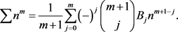 (1.4)
(1.4)
This famous conjectured formula of Bernoulli was proven in 1755 based on the calculus of finite difference by Euler [7] , a researcher working with the Bernoulli brothers at Zurich. As informed by Raugh [8] , Euler had followed de Moivre in given the denomination Bernoulli numbers, introduced the Bernoulli polynomials in 1738 via the generating function
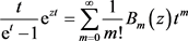 (1.5)
(1.5)
Returning to the Faulhaber conjecture saying that is a polynomial in for all m
 (1.6)
(1.6)
we know that Jacobi [9] has the merit of giving the right proof for this conjecture and moreover calculating the first six Faulhaber coefficients although he did not get a formula for obtaining all of them. Another merit of Jacobi consists in pioneering the use of the derivative with respect to n when observing that
 (1.7)
(1.7)
(1.8)
Long years passed until Edwards [10] showed how to obtain the Faulhaber coefficients by matrix inversion and Knuth [4] by identification of coefficients of odd powers of n in Bernoulli formula with those in Faulhaber conjecture. Nevertheless the methods of Edwards and Knuth are not easy to apply.
Following Coen, we know the existence of the work Bernoulli numbers: bibliography (1713-1990) of Dilcher [11] which contained 1956 references by 839 authors!
Concerning the more general problem of powers sums on arithmetic progressions
 (1.9)
(1.9)
we remark the recent formula given by Dattoli, Cesarano, Lorenzutta [12] in term of Bernoulli polynomials
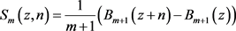 (1.10)
and the formula of Chen, Fu, Zhang [13] in term of sums of powers of
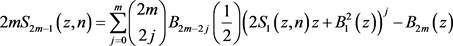 (1.11)
which are not easy to apply.
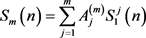
After these authors we have proposed a method leading to the formula [14]
 (1.12)
where and .
The Faulhaber formula is thus obtained but we see that the method for obtaining it is cumbersome and the practice calculations of for obtaining the Faulhaber coefficients fastidious.
Rethinking the problem, we observe that an arithmetic progression is a matter of translation, that there is a somehow symmetry between and and so that finally we found a more concise method for resolving the problem and theoretically and practically that we will expose in the following paragraphs.
2. Representation of a Power Sums and Bernoulli Polynomials by Differential Operators
Let
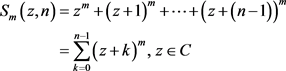 (2.1)
(2.1)
be the powers sums on an arithmetic progression and
 (2.2)
(2.2)
the powers sums of the first integers.
We may utilize the shift or translation operator
 (2.3)
(2.3)
to get the differential representation
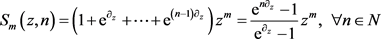 (2.4)
(2.4)
which gives directly the relations
 (2.5)
(2.5)
 (2.6)
(2.6)
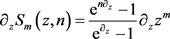
and the generating function
 (2.7)
(2.7)
Because (2.4) is valid for all integers n it is also valid for all real and complex values so that we may write
 (2.8)
(2.8)
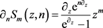
Defining now the set of polynomials by the differential representation
 (2.9)
(2.9)
we see that verify
 (2.10)
 (2.11)
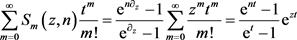
and have the generating function
 (2.12)
allowing the identification of them with Bernoulli polynomials defined by Euler [7] and giving the first of them
, . (2.13)
The Bernoulli polynomials are linked to powers sums according to formulae (2.5), (2.8), (2.9) by the relations
 (2.14)
 (2.15)
which lead to the followed beautiful formula where the second member does not depend on n
 (2.16)
Besides it leads also to the formula
 (2.17)
which jointed with (2.15) gives rise to the historic Jacobi conjectured formula [9]
 (2.18)
From (2.18) we see that are identifiable with Bernoulli numbers .
3. The Powers Sums
1) Powers sums in terms of Bernoulli polynomials and powers of n
From the Equation (2.16) and the boundary condition we get immediately the solution of (2.16)
(3.1)
which may be put under the algorithmic form very easy to remember
 (3.2)
(3.2)
or taking into account (2.11)
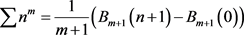
Putting in (3.2) and replacing with we recognize the famous Bernoulli formula [6]
 (3.3)
(3.3)
2) The Faulhaber formula on powers sums
In instead of utilizing z and n for arguments let us utilize
and (3.4)
Because
 (3.5)
(3.5)
we have
 (3.6)
(3.6)
 (3.7)
(3.7)
(3.8)
Equation (2.16) becomes
 (3.9)
(3.9)
Happily from the definition of by differential operators (2.9) we may write down
(3.10)
which jointed with (2.10) leads to the important properties
 (3.11)
 (3.12)
 (3.13)
As an polynomial of order 2k having for roots may be put by identification of coefficients under the form of a homogeneous polynomial of order k in we obtain the important property:
is a homogeneous polynomial of order k in (3.14)
By the way we notify that because for it is also a homogeneous polynomial of order in as conjectured Faulhaber and proven somehow by Jacobi.
Moreover the calculations of the quoted polynomials in Z or in u may be done thank to the hereinafter Table 3.
Jointed (3.14) with the formula came from the Jacobi formula (2.18)
 (3.15)
we may define a polynomial of order k depending on Z such that
 (3.16)
 (3.17)
The definition of by (3.16) differs a little in index with its definition in [15] .
Thank to these considerations we get the solution of (3.9) corresponding to the boundary condition under the form
(3.18)
or under the algorithmic form
 (3.19)
where we see that the Faulhaber coefficients are successive derivations beginning from the first one of the power sums on integers writing under the form .
Curiously by replacing z with n and consequently Z with in the definition we get the very important and very interesting formula linking the Faulhaber powers sums on integers and on arithmetic progressions
 (3.20)
For examples
 (3.21)
 (3.22)
4. Obtaining Practically Bernoulli Numbers, Bernoulli Functions and Powers Sums
4.1. Calculations of Bernoulli Numbers
For calculating we remark that from
 (4.1)
(4.1)
and (2.10) we get the recursion relation
 (4.2)
(4.2)
which may be written under the matrix form
(4.3)
This matrix equation may be resolved by doing by hand or by program linear combinations over lines from the second one in order to replace them with lines each containing only some non-zero rational numbers.
For instance for calculating successively  we may utilize the matrix equation
Matrix equation for calculating .

 =
=  (4.4)
(4.4)
We remark that the last line of this matrix has replaced the line  Some results are
,,,

4.2. Calculations of Bernoulli Polynomials
For calculating Bernoulli polynomials, we remark that (2.11) and the Jacobi formula (2.18) give rise to the relations
 (4.5)
(4.5)
 (4.6)
(4.6)
which, knowing , permits the easy calculations of all the Bernoulli polynomials and the powers sums on integers
  from the set of Bernoulli numbers
  as we may see hereafter in Table 1.
4.3. Calculations of Powers Sums as Polynomials in n
For calculating we utilize the algorithmic formula (3.2) and get the results shown in Table 2.
4.4. Calculations of Faulhaber Powers Sums
Practically for transforming into from which one obtains the Faulhaber coefficients let us remark that
 (4.7)
(4.7)
so that we may replace the first term of with minus a polynomial in z. The polynomial in z so obtained must begin with a term in and not so that we may continue to replace in it with a term in
Table 1. Obtaining , from .
Table 2. Obtaining from .
minus a polynomial in z. The operations continue so on until finish.
By this operation we observe that we may omit all odd powers terms in before and during the transformation of into for . From these remarks we may establish Table 3 of transformation.
This algorithm for obtaining gives rise astonishingly to the easy calculation of the Faulhaber formula for .
As examples we have
・
 (4.8)
(4.8)
・
Table 3. Change of  in change of
  into
into .
.

(4.9)
・
(4.10)
・
(4.11)
5. Formula for Even Powers Sums
By derivation of with respect to z and remarking that
, (5.1)
we obtain the formulae giving in function of
(5.2)
(5.3)
(5.4)
For examples
・ ,,
(5.5)
・
(5.6)
6. Remarks and Conclusions
The main particularity of this work consists in obtaining as the transform of by a differential operator, as so as the Bernoulli polynomial , from which we deduce the new formula and get immediately as polynomials in n. From which we get also the property saying that is a homogeneous polynomial of order k in .
The second particularity consists in performing the change of arguments from z into and n into in order to get the relation which gives rise to the Faulhaber formula of . From this formula we see that the Faulhaber coefficients are successive derivatives of the function where are powers sums on integers.
The relation leads also to the Faulhaber formula where .
The third particularity of this work is proposing a method for obtaining easily the Bernoulli numbers from a matrix equation, then of
.
As conclusion we think that the calculations of powers sums are greatly facilitated by the utilization of derivation operators and the translation operator , parts of Operator Calculus.
Operator calculus, which is very different from Heaviside operational calculus, is thus merited to be known and introduced into Mathematical Analysis. Moreover it just had a solid foundation and many interesting applications for instance in the domains of Special functions, Differential equations, Fourier, Laplace and other transforms, quantum mechanics [14] .
Acknowledgements
The author acknowledges the reviewer for comments leading to the clear proof of the important formula (3.14). The author also acknowledges Mrs. Beverly GUO for her perseverance in the refinement of the article representation.
He reiterates his gratitude toward his adorable wife for all the cares she devoted for him during the long months he performed this work.
Conflicts of Interest
The author declares no conflicts of interest regarding the publication of this paper.
Cite this paper
Si, D.T. (2019) The Powers Sums, Bernoulli Numbers, Bernoulli Polynomials Rethinked. Applied Mathematics, 10, 100-112. https://doi.org/10.4236/am.2019.103009
References
- 1. Coen, L.E.S. (1996) Sums of Powers and the Bernoulli Numbers. Master’s Thesis, Eastern Illinois University, Charleston, IL.
https://thekeep.eiu.edu/theses/1896/ - 2. Edwards, A.W.F. (1982) Sums of Powers of Integers: A Little of the History, The Mathematical Gazette, 66, 22-28.
https://www.jstor.org/stable/3617302 - 3. Faulhaber, J. (1631) Academia Algebrae, Augspurg, Call Number QA154.8 F3 1631a f MATH at Stanford University Libraries. Johann Ulrich Schonigs, Augspurg.
- 4. Knuth, D.E. (1993) Johann Faulhaber and Sums of Powers. Mathematics of Computation, 61, 277-294.
https://doi.org/10.1090/S0025-5718-1993-1197512-7 - 5. Beardon, A.F. (1996) Sums of Powers of Integers. The American Mathematical Monthly, 103, 201-213.
https://doi.org/10.1080/00029890.1996.12004725 - 6. Bernoulli, J. (1713) Ars Conjectandi, Was Published Posthumously in Euler L. (1738).
- 7. Euler, L. (1738) Methodus generalis summandi progressiones. In: Commentarii academiae scientiarum Petropolitanae 6, 1738, 68-97.
- 8. Raugh, M. (2014) The Bernoulli Summation Formula: A Pretty Natural Derivation. A Presentation for Los Angeles City College at The High School Math Contest.
http://www.mikeraugh.org/ - 9. Jacobi, C.G.J. (1834) De usu legitimo formulae summatoriae Maclaurinianae. Journal für die Reine und Angewandte Mathematik, 1834, 263-272.
https://doi.org/10.1515/crll.1834.12.263 - 10. Edwards, A.W.F. (1986) A Quick Route to Sums of Powers. The American Mathematical Monthly, 93, 451-455.
https://doi.org/10.1080/00029890.1986.11971850 - 11. Dilcher, K., Shula, L. and Slavutskii, I. (1991) Bernoulli Numbers Bibliography (1713-1990). Queen’s Papers in Pure and Applied Mathematics, No. 87.
- 12. Dattoli, G., Cesarano, C. and Lorenzutta, S. (2002) Bernoulli Numbers and Polynomials from a More General Point of View. Rendiconti di Matematica, 22, 193-202.
- 13. Chen, W.Y.C., Fu, A.M. and Zhang, I.F. (2009) Faulhaber’s Theorem on Power Sums. Discrete Mathematics, 309, 2974-2981.
https://doi.org/10.1016/j.disc.2008.07.027 - 14. Do, T.S. (2016) Operator Calculus. Lambert Academic Publishing, Sarrbrücken, Germany.
- 15. Do, T.S. (2018) The Faulhaber Problem on Sums of Powers on Arithmetic Progressions Resolved. Applied Physics Research, 10, 5-20.
https://doi.org/10.5539/apr.v10n2p5