ABSTRACT

We show that Yang-Mills equation in 3 dimensions is local well-posedness in $H^s$ if the norm is sufficiently. Here, we construct a solution on the quadric that is independent of the time. And we also construct a solution of the polynomial form. In the process of solving, the polynomial is used to solve the problem before solving.

Keywords:

$H^s$ -Space, Well-Posedness, Polynomial, Quadric

1. Introduction and Preliminaries

This paper is concerned with the solution of the Yang-Mills equation.

We shall denote $g$ -valued tensors define on Minkowski space-time

$A_{\alpha }:R^{3+1}\to g$ by bold character $A_{\alpha }$ , where $\alpha$ ranges over 0, 1, 2, 3. We use the usual summation conventions on $\alpha$ , and raise and lower indices with respect to the Minkowski metric ${\eta }^{\alpha \beta }:=\text{diag}\left(-1,1,1,1\right)$ ; for more details, see [1] [2] [3] . Given an arbitrary $g$ -valued tensor $F_{\alpha \beta }:R^{3+1}\to g$ .

The curvature of a connection $F_{\alpha \beta }$ by

$F_{\alpha \beta }:={\partial }_{\alpha }{A}_{\beta }-{\partial }_{\beta }{A}_{\alpha }+\left[A_{\alpha },A_{\beta }\right]$

Here [,] denotes the Lie bracket of $g$ . It appears in calculations whenever we commute covariant derivatives [4] [5] , or more precisely that

${\partial }_{\alpha }{F}^{\alpha \beta }+\left[A_{\alpha },F^{\alpha \beta }\right]=0$

We can expand this as

$\square A^{\beta }-{\partial }^{\beta }\left({\partial }_{\alpha }{A}^{\beta }\right)+\left[A_{\alpha },{\partial }^{\alpha }{A}^{\beta }\right]-\left[A_{\alpha },{\partial }^{\beta }{A}^{\alpha }\right]+\left[A_{\alpha },\left[A^{\alpha },A^{\beta }\right]\right]=0$

where $\square :=-{\partial }_t^2+\Delta ,\alpha ,\beta =0,1,2,3.$

The Cauchy problem for Yang-mills equation is not well-posed because of gauge invariance (see [6] [7] ). However, if one fixes the connection to lie in the temporal gauge $A_0=0$ , the Yang-Mills equations become essentially hyperbolic [8] [9] , and simplify to

${\partial }_t\left(\text{div}A\right)+\left[A_i,{\partial }_t{A}_i\right]=0$ (1)

and

$\square A_j-{\partial }_j\left(\text{div}A\right)++\left[A_i,{\partial }_i{A}_j\right]-\left[A_i,{\partial }_j{A}_i\right]+\left[A_i,\left[A_i,A_j\right]\right]=0$ (2)

where $i,j=1,2,3$ .

The local well-posedness of the Equations (1) and (2) have already proved in [10] . Here in not described in detail. This paper will show that the solution of operator and polynomial type.

2. Exact Solution of Equation

Below we will construct the exact solution of the equation on the general quadric that denotes by

$A_i={\partial }_{x_i}+a_{i}i=1,2,3.$ (3)

where $a_i=a_i\left(x_1,x_2,x_3\right)$ .

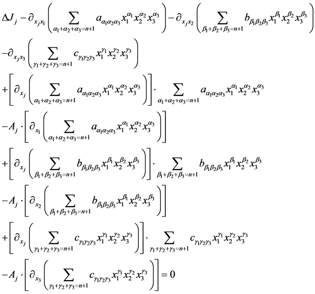
We bring (3) to Equation (2), because the equation is used in the two general surfaces, we define the general quadric by

$f={\displaystyle \sum _{{\alpha }_1+{\alpha }_2+{\alpha }_3\le 2}{c}_{{\alpha }_1{\alpha }_2{\alpha }_3}{x}_1^{{\alpha }_1}{x}_2^{{\alpha }_2}{x}_3^{{\alpha }_3}}$

${\alpha }_1,{\alpha }_2,{\alpha }_3=0,1,2.c_{{\alpha }_1{\alpha }_2{\alpha }_3}$ as coefficient and $c_{{\alpha }_1{\alpha }_2{\alpha }_3}\in R$ . So we calculate the equation. The first calculation can be

Finally, the sections of Lie bracket can be

$\begin{array}{c}\left[A_i,{\partial }_i{A}_j\right]f=\left[\left(A_i\cdot {\partial }_i{A}_j-{\partial }_i{A}_j\cdot A_i\right)\right]f\\ =\left[\left({\partial }_{x_i}+a_i\right)\left({\partial }_{x_j}{\partial }_{x_i}+\frac{\partial a_j}{{\partial }_{x_i}}+a_j{\partial }_{x_i}\right)-\left({\partial }_{x_j}{\partial }_{x_i}+\frac{\partial a_j}{{\partial }_{x_i}}+a_j{\partial }_{x_i}\right)\left({\partial }_{x_i}+a_i\right)\right]f\\ =\left(\frac{{\partial }^2{a}_j}{{\partial }_{x_i}{\partial }_{x_i}}+\frac{\partial a_j}{{\partial }_{x_i}}{\partial }_{x_i}-\frac{{\partial }^2{a}_i}{{\partial }_{x_j}{\partial }_{x_i}}-\frac{\partial a_i}{{\partial }_{x_i}}{\partial }_{x_j}-\frac{\partial a_i}{{\partial }_{x_j}}{\partial }_{x_i}-a_j\frac{\partial a_i}{{\partial }_{x_i}}\right)f\\ =(\frac{{\partial }^2{a}_j}{{\partial }_{x_i}{\partial }_{x_i}}-a_j\frac{\partial a_i}{{\partial }_{x_i}}-\frac{\partial a_i}{{\partial }_{x_i}}{\partial }_{x_j})f+(\frac{\partial a_j}{{\partial }_{x_1}}+\frac{\partial a_1}{{\partial }_{x_1}})\left(c_{100}+c_{110}{x}_2+c_{101}{x}_3+2c_{200}{x}_1\right)\\ =(\frac{\partial a_j}{{\partial }_{x_2}}+\frac{\partial a_2}{{\partial }_{x_2}})\left(c_{010}+c_{110}{x}_1+c_{011}{x}_3+2c_{020}{x}_2\right)+(\frac{\partial a_j}{{\partial }_{x_3}}+\frac{\partial a_3}{{\partial }_{x_3}})(c_{001}+c_{101}{x}_1\\ +c_{011}{x}_2+2c_{002}{x}_3)\end{array}$

$\begin{array}{c}\left[A_i,{\partial }_j{A}_i\right]f=\left[\left(A_i\cdot {\partial }_j{A}_i-{\partial }_j{A}_i\cdot A_i\right)\right]f\\ =\left[\left({\partial }_{x_i}+a_i\right)\left({\partial }_{x_j}{\partial }_{x_i}+\frac{\partial a_i}{{\partial }_{x_j}}+a_i{\partial }_{x_j}\right)-\left({\partial }_{x_j}{\partial }_{x_i}+\frac{\partial a_i}{{\partial }_{x_j}}+a_i{\partial }_{x_j}\right)\left({\partial }_{x_i}+a_i\right)\right]f\\ =-\left(\frac{\partial a_i}{{\partial }_{x_j}}{\partial }_{x_i}+a_i\frac{\partial a_i}{{\partial }_{x_j}}\right)f\\ =-[\frac{\partial a_1}{{\partial }_{x_j}}\left(c_{100}+c_{110}{x}_2+c_{101}{x}_3+2c_{200}{x}_1\right)+\frac{\partial a_2}{{\partial }_{x_j}}\left(c_{010}+c_{110}{x}_1+c_{011}{x}_3+2c_{020}{x}_2\right)\\ +\frac{\partial a_3}{{\partial }_{x_j}}\left(c_{001}+c_{101}{x}_1+c_{011}{x}_2+2c_{002}{x}_3\right)+(a_1\frac{\partial a_1}{{\partial }_{x_j}}+a_2\frac{\partial a_2}{{\partial }_{x_j}}+a_3\frac{\partial a_3}{{\partial }_{x_j}})f]\end{array}$

$\begin{array}{c}\left[A_i,\left[A_i,A_j\right]\right]f=\left[A_i,A_i{A}_j-A_j{A}_i\right]f\\ =\left[A_i,\left({\partial }_{x_i}+a_i\right)\left({\partial }_{x_j}+a_j\right)-\left({\partial }_{x_j}+a_j\right)\left({\partial }_{x_i}+a_i\right)\right]f\\ =\left[A_i,\frac{\partial a_j}{{\partial }_{x_i}}-\frac{\partial a_i}{{\partial }_{x_j}}\right]f\\ =\left[\left({\partial }_{x_i}+a_i\right)\left(\frac{\partial a_j}{{\partial }_{x_i}}-\frac{\partial a_i}{{\partial }_{x_j}}\right)-\left(\frac{\partial a_j}{{\partial }_{x_i}}-\frac{\partial a_i}{{\partial }_{x_j}}\right)\left({\partial }_{x_i}+a_i\right)\right]f\\ =\left(\frac{{\partial }^2{a}_j}{{\partial }_{x_i}{\partial }_{x_i}}-\frac{{\partial }^2{a}_i}{{\partial }_{x_j}{\partial }_{x_i}}\right)f\end{array}$

Combining the above calculations we have

$\begin{array}{l}2a_j\left(c_{200}+c_{020}+c_{002}\right)+[\Delta a_j-\frac{{\partial }^2{a}_j}{\partial t^2}+2\frac{{\partial }^2{a}_j}{\partial x_i^2}-2\left(\frac{{\partial }^2{a}_1}{\partial x_j\partial x_1}+\frac{{\partial }^2{a}_2}{\partial x_j\partial x_2}+\frac{{\partial }^2{a}_3}{\partial x_j\partial x_3}\right)\\ +a_j\left(\frac{\partial a_1}{\partial x_1}+\frac{\partial a_2}{\partial x_2}+\frac{\partial a_3}{\partial x_3}\right)+a_1\frac{\partial a_1}{\partial x_j}+a_2\frac{\partial a_2}{\partial x_j}+a_3\frac{\partial a_3}{\partial x_j}]f+\frac{\partial a_j}{\partial x_1}(c_{100}+c_{110}{x}_2+c_{101}{x}_3\\ +2c_{200}{x}_1)+\frac{\partial a_j}{\partial x_2}\left(c_{010}+c_{110}{x}_1+c_{011}{x}_3+2c_{020}{x}_2\right)+\frac{\partial a_j}{\partial x_3}(c_{001}+c_{101}{x}_1+c_{011}{x}_2\\ +2c_{002}{x}_3)-\left(\frac{\partial a_1}{\partial x_1}\partial x_j+\frac{\partial a_2}{\partial x_2}\partial x_j+\frac{\partial a_3}{\partial x_3}\partial x_j\right)f=0\end{array}$

We will use the properties of polynomials to list the coefficient equations in order to solve the (3). For the cross terms and square terms coefficient, we have

$\begin{array}{l}\Delta a_j-\frac{{\partial }^2{a}_j}{\partial t^2}+2\frac{{\partial }^2{a}_j}{\partial x_i^2}-2\left(\frac{{\partial }^2{a}_1}{\partial x_j\partial x_1}+\frac{{\partial }^2{a}_2}{\partial x_j\partial x_2}+\frac{{\partial }^2{a}_3}{\partial x_j\partial x_3}\right)\\ +a_j\left(\frac{\partial a_1}{\partial x_1}+\frac{\partial a_2}{\partial x_2}+\frac{\partial a_3}{\partial x_3}\right)+a_1\frac{\partial a_1}{\partial x_j}+a_2\frac{\partial a_2}{\partial x_j}+a_3\frac{\partial a_3}{\partial x_j}=0\end{array}$ (4)

First, we consider $j=1$ .

The constant coefficient equation is

$\begin{array}{l}2a_1\left(c_{200}+c_{020}+c_{002}\right)+\Delta a_1-\frac{{\partial }^2{a}_1}{\partial t^2}+2\frac{{\partial }^2{a}_1}{\partial x_i^2}-2\left(\frac{{\partial }^2{a}_1}{\partial x_1\partial x_1}+\frac{{\partial }^2{a}_2}{\partial x_1\partial x_2}+\frac{{\partial }^2{a}_3}{\partial x_1\partial x_3}\right)\\ +a_1\left(\frac{\partial a_1}{\partial x_1}+\frac{\partial a_2}{\partial x_2}+\frac{\partial a_3}{\partial x_3}\right)+a_1\frac{\partial a_1}{\partial x_1}+a_2\frac{\partial a_2}{\partial x_1}+a_3\frac{\partial a_3}{\partial x_1}+\frac{\partial a_1}{\partial x_1}{c}_{100}\\ +\frac{\partial a_2}{\partial x_2}{c}_{010}+\frac{\partial a_3}{\partial x_3}{c}_{001}-\left(\frac{\partial a_1}{\partial x_1}+\frac{\partial a_2}{\partial x_2}+\frac{\partial a_3}{\partial x_3}\right)c_{100}=0\end{array}$

The coefficient equation of $x_1$ is

$\frac{\partial a_1}{\partial x_2}{c}_{110}+\frac{\partial a_1}{\partial x_3}{c}_{101}-2\frac{\partial a_2}{\partial x_2}{c}_{200}-2\frac{\partial a_3}{\partial x_3}{c}_{200}=0$ (5)

The coefficient equation of $x_2$ is

$2\frac{\partial a_1}{\partial x_2}{c}_{020}+\frac{\partial a_1}{\partial x_3}{c}_{011}-\frac{\partial a_2}{\partial x_2}{c}_{110}-\frac{\partial a_3}{\partial x_3}{c}_{110}=0$ (6)

The coefficient equation of $x_3$ is

$\frac{\partial a_1}{\partial x_2}{c}_{011}+2\frac{\partial a_1}{\partial x_3}{c}_{002}-\frac{\partial a_2}{\partial x_2}{c}_{101}-\frac{\partial a_3}{\partial x_3}{c}_{101}=0$ (7)

Because of the (4), the coefficient equation of constant can be

$2a_1\left(c_{200}+c_{020}+c_{002}\right)+\frac{\partial a_1}{\partial x_2}{c}_{010}+\frac{\partial a_1}{\partial x_3}{c}_{001}-\frac{\partial a_2}{\partial x_2}{c}_{100}-\frac{\partial a_3}{\partial x_3}{c}_{100}=0$ (8)

$\left(6\right)\times c_{110}\times c_{101}-\left(7\right)\times c_{200}\times c_{101}-\left(8\right)\times c_{200}\times c_{110}$ we have

$\begin{array}{l}\frac{\partial a_1}{\partial x_2}\left(c_{110}{c}_{110}{c}_{101}-2c_{020}{c}_{200}{c}_{101}-c_{011}{c}_{200}{c}_{110}\right)\\ +\frac{\partial a_1}{\partial x_3}\left(c_{101}{c}_{110}{c}_{101}-c_{011}{c}_{200}{c}_{101}-2c_{020}{c}_{011}{c}_{200}\right)=0\end{array}$ (9)

Deformation by (6), we have

$\frac{\partial a_2}{\partial x_2}+\frac{\partial a_3}{\partial x_3}=2\frac{\partial a_1}{\partial x_2}{c}_{020}+\frac{\partial a_1}{\partial x_3}{c}_{011}/c_{110}$ (10)

Simulaneous (8) and (10), we have

$2a_1\left(c_{200}+c_{020}+c_{002}\right)+\frac{\partial a_1}{\partial x_2}\left(c_{010}-2\frac{c_{020}{c}_{100}}{c_{110}}\right)+\frac{\partial a_1}{\partial x_3}\left(c_{001}-\frac{c_{011}{c}_{100}}{c_{110}}\right)=0$ (11)

First, for (9) we can use mathematica to get

$\begin{array}{l}{a}_1=C_1\left[x_1\right]\\ \left[\frac{-\left(c_{101}{c}_{110}{c}_{101}-c_{011}{c}_{200}{c}_{101}-2c_{020}{c}_{011}{c}_{200}\right)x_2+\left(c_{110}{c}_{110}{c}_{101}-2c_{020}{c}_{200}{c}_{101}-c_{011}{c}_{200}{c}_{110}\right)x_3}{c_{110}{c}_{110}{c}_{101}-2c_{020}{c}_{200}{c}_{101}-c_{011}{c}_{200}{c}_{110}}\right]\end{array}$

where $C_1$ is a constant, $\left[\right]$ denotes the arbitrary combination of functions represented as independent variables in square brackets. For example, $\left[x\right]$ is represented as $x\sin x$ or $e^x\ln x\cos x$ and so on.

Next, from (11) we can obtain

$a_1=C_2{e}^{\frac{2\left(c_{200}+c_{020}+c_{002}\right)x_2}{c_{010}-2c_{020}{c}_{100}/c_{110}}}\left[x_1\right]\left[\frac{-\left(c_{001}-c_{011}{c}_{100}/c_{110}\right)x_2+\left(c_{010}-2c_{020}{c}_{100}/c_{110}\right)x_3}{c_{010}-2c_{020}{c}_{100}/c_{110}}\right]$

where $C_2$ is a constant.

We can observe the above $a_1$ and the general properties of two surfaces, $a_1$ is irrelevant to the $x_{\text{2}}$ and $x_{\text{3}}$ , so $a_1=a_1\left(x_1\right)$ .

Because of $a_1=a_1\left(x_1\right)$ , we take $a_1$ into the (11) can be obtain

$2a_1\left(c_{200}+c_{020}+c_{002}\right)=0$

By two surfaces we can obtain

$a_1=0$

Similarly, we can prove that $j=2,3$ , we have

$a_2,a_3=0$

In summary, when the Equation (2) is acting on the quadric, we have

$\{\begin{array}{c}{A}_1={\partial }_{x_1}\\ A_2={\partial }_{x_2}\\ A_3={\partial }_{x_3}\end{array}$

3. Polynomial Solutions

3.1. First Order Polynomial Solution

Below we construct a polynomial solution. First, the constant must satisfy the equation so that all constant are the solutions of the Equation (1) and (2). Then we define the solution of a polynomial form on a surface by

$A_i=a_i{x}_1+b_i{x}_2+c_i{x}_3+d_i$

where $i=1,2,3$ , $A_i$ is satisfied the (1) because of not contain time t. Then we just need to bring $A_i$ into (2). We have

$\Delta A_j-{\partial }_j\left(\text{div}A\right)+{\displaystyle \sum _{i=1}^3\left({\partial }_j{A}_i{A}_i-A_j{\partial }_i{A}_i\right)}=0$ (12)

Equation (12) is composed of three equations. First we consider the case of $j=1$ . So the constant coefficient equation is

$b_2{d}_2-b_2{d}_1+a_3{d}_3-c_3{d}_1=0$

The coefficient equation of $x_1$ is

$a_2{b}_2-a_1{b}_2+a_3{a}_3-a_1{c}_3=0$

The coefficient equation of $x_2$ is

$b_2{b}_2-b_1{b}_2+a_3{b}_3-b_1{c}_3=0$

The coefficient equation of $x_3$ is

$b_2{c}_2-b_2{c}_1+a_3{c}_3-c_1{c}_3=0$

When $j=2$ , the relationship of the coefficients are

$\{\begin{array}{l}{b}_1{d}_1-a_1{d}_2+c_3{d}_3-c_3{d}_2=0\hfill \\ a_1{b}_1-a_1{a}_2+a_3{c}_3-a_2{c}_3=0\hfill \\ b_1{b}_1-a_1{b}_2+b_3{c}_3-b_2{c}_3=0\hfill \\ b_1{c}_1-a_1{c}_2+c_3{c}_3-c_2{c}_3=0\hfill \end{array}$

When $j=3$ , the relationship of the coefficients are

$\{\begin{array}{l}{c}_1{d}_1-a_1{d}_3+c_2{d}_2-b_2{d}_3=0\hfill \\ a_1{c}_1-a_1{a}_3+a_2{c}_2-a_2{b}_3=0\hfill \\ b_1{c}_1-a_1{b}_3+b_2{c}_2-b_2{b}_3=0\hfill \\ c_1{c}_1-a_1{c}_3+c_2{c}_2-b_2{c}_3=0\hfill \end{array}$

There exist 12 equations. By solving the above equations, we can obtain

$a_1=a_2=a_3=b_1=b_2=b_3=c_1=c_2=c_3$

$d_1=d_2=d_3$

Therefore

$A_i=a{x}_1+a{x}_2+a{x}_3+b$ (13)

where $a,b\in Ri=1,2,3$ .

In summary, the solution of the polynomial form of Yang-Mills equation is expressed in the form of (13).

3.2. The Quadratic Polynomial Solution

In this section, we mainly discuss the solution of the quadratic polynomial form of the Yang-Mills equation on the two surfaces. We define by

$\{\begin{array}{l}{A}_1={\displaystyle \sum _{{\alpha }_1+{\alpha }_2+{\alpha }_3\le 2}{a}_{{\alpha }_1{\alpha }_2{\alpha }_3}{x}_1^{{\alpha }_1}}{x}_2^{{\alpha }_2}{x}_3^{{\alpha }_3}\hfill \\ A_2={\displaystyle \sum _{{\beta }_1+{\beta }_2+{\beta }_3\le 2}{b}_{{\beta }_1{\beta }_2{\beta }_3}{x}_1^{{\beta }_1}}{x}_2^{{\beta }_2}{x}_3^{{\beta }_3}\hfill \\ A_3={\displaystyle \sum _{{\gamma }_1+{\gamma }_2+{\gamma }_3\le 2}{c}_{{\gamma }_1{\gamma }_2{\gamma }_3}{x}_1^{{\gamma }_1}}{x}_2^{{\gamma }_2}{x}_3^{{\gamma }_3}\hfill \end{array}$

where ${\alpha }_i,{\beta }_i,{\gamma }_i\in \mathbb{N}i=1,2,3$ , $a_{{\alpha }_1{\alpha }_2{\alpha }_3},b_{{\beta }_1{\beta }_2{\beta }_3},c_{{\gamma }_1{\gamma }_2{\gamma }_3}\in R$ are coefficients. So

$A_1,A_2,A_3$ must satisfy the Equation (1), therefore, it just needs to take

$A_1,A_2,A_3$ into (12), we have

There exist 30 equations and 30 unknowns. Solving the equations we can obtain the following results

$a_{200}=a_{020}=a_{002}=a_{110}=a_{101}=a_{011}=0$

$b_{200}=b_{020}=b_{002}=b_{110}=b_{101}=b_{011}=0$

$c_{200}=c_{020}=c_{002}=c_{110}=c_{101}=c_{011}=0$

$a_{100}=a_{010}=a_{011}=b_{100}=b_{010}=b_{001}=c_{100}=c_{010}=c_{001}\in ℝ$

$a_{000}=b_{000}=c_{000}\in ℝ$

So the solution of the equation can be written

$A_i=a{x}_1+a{x}_2+a{x}_3+b$ (14)

where $a,b\in ℝi=1,2,3.$

In summary, the solution of the quadratic polynomial form of Yang-Mills equation is (14). It obvious that (13) is equal to (14). So we conjecture that the solution of n-degree polynomial on n-sub surface is also (14). In the next section, we will proof the hypothesis.

3.3. Solution of N-Degree Polynomial

In this section, we mainly use mathematical induction to prove the hypothesis. We define that by

$\{\begin{array}{l}{A}_1={\displaystyle \sum _{{\alpha }_1+{\alpha }_2+{\alpha }_3\le n}{a}_{{\alpha }_1{\alpha }_2{\alpha }_3}{x}_1^{{\alpha }_1}}{x}_2^{{\alpha }_2}{x}_3^{{\alpha }_3}\hfill \\ A_2={\displaystyle \sum _{{\beta }_1+{\beta }_2+{\beta }_3\le n}{b}_{{\beta }_1{\beta }_2{\beta }_3}{x}_1^{{\beta }_1}}{x}_2^{{\beta }_2}{x}_3^{{\beta }_3}\hfill \\ A_3={\displaystyle \sum _{{\gamma }_1+{\gamma }_2+{\gamma }_3\le n}{c}_{{\gamma }_1{\gamma }_2{\gamma }_3}{x}_1^{{\gamma }_1}}{x}_2^{{\gamma }_2}{x}_3^{{\gamma }_3}\hfill \end{array}$ (15)

where ${\alpha }_i,{\beta }_i,{\gamma }_i\in \mathbb{N}i=1,2,3$ , $a_{\alpha },b_{\beta },c_{\gamma }\in R$ are coefficients.

In the front two sections, it is easy for us to conclude that when $n=1,2$ the solutions are the same. So we will use mathematical induction to prove that when $n\ge 2$ the solution is also (14).

First, we assume that when $n\left(n\ge 2\right)$ the solution of the equation is

$A_i=a{x}_1+a{x}_2+a{x}_3+b$

where $a,b\in ℝi=1,2,3.$

Now when $n+1$ , we h ave

To further simplify (15), we have

$\{\begin{array}{l}{A}_1={\displaystyle \sum _{{\alpha }_1+{\alpha }_2+{\alpha }_3\le n}{a}_{{\alpha }_1{\alpha }_2{\alpha }_3}{x}_1^{{\alpha }_1}}{x}_2^{{\alpha }_2}{x}_3^{{\alpha }_3}+{\displaystyle \sum _{{\alpha }_1+{\alpha }_2+{\alpha }_3=n+1}{a}_{{\alpha }_1{\alpha }_2{\alpha }_3}{x}_1^{{\alpha }_1}}{x}_2^{{\alpha }_2}{x}_3^{{\alpha }_3}\hfill \\ A_2={\displaystyle \sum _{{\beta }_1+{\beta }_2+{\beta }_3\le n}{b}_{{\beta }_1{\beta }_2{\beta }_3}{x}_1^{{\beta }_1}}{x}_2^{{\beta }_2}{x}_3^{{\beta }_3}+{\displaystyle \sum _{{\beta }_1+{\beta }_2+{\beta }_3=n+1}{b}_{{\beta }_1{\beta }_2{\beta }_3}{x}_1^{{\beta }_1}}{x}_2^{{\beta }_2}{x}_3^{{\beta }_3}\hfill \\ A_3={\displaystyle \sum _{{\gamma }_1+{\gamma }_2+{\gamma }_3\le n}{c}_{{\gamma }_1{\gamma }_2{\gamma }_3}{x}_1^{{\gamma }_1}}{x}_2^{{\gamma }_2}{x}_3^{{\gamma }_3}+{\displaystyle \sum _{{\gamma }_1+{\gamma }_2+{\gamma }_3=n+1}{c}_{{\gamma }_1{\gamma }_2{\gamma }_3}{x}_1^{{\gamma }_1}}{x}_2^{{\gamma }_2}{x}_3^{{\gamma }_3}\hfill \end{array}$

To bring into the equation, we have

where $J_j$ is

$\{\begin{array}{l}{J}_1={\displaystyle \sum _{{\alpha }_1+{\alpha }_2+{\alpha }_3=n+1}{a}_{{\alpha }_1{\alpha }_2{\alpha }_3}{x}_1^{{\alpha }_1}}{x}_2^{{\alpha }_2}{x}_3^{{\alpha }_3}\hfill \\ J_2={\displaystyle \sum _{{\beta }_1+{\beta }_2+{\beta }_3=n+1}{b}_{{\beta }_1{\beta }_2{\beta }_3}{x}_1^{{\beta }_1}}{x}_2^{{\beta }_2}{x}_3^{{\beta }_3}\hfill \\ J_3={\displaystyle \sum _{{\gamma }_1+{\gamma }_2+{\gamma }_3=n+1}{c}_{{\gamma }_1{\gamma }_2{\gamma }_3}{x}_1^{{\gamma }_1}}{x}_2^{{\gamma }_2}{x}_3^{{\gamma }_3}\hfill \end{array}$

On the number of $x$ in the above equation is either less than $n$ , or more than $n+1$ . When the number of $x$ is less than $n$ , the solution of the equation is

$A_i=a{x}_1+a{x}_2+a{x}_3+b$

And the number of more than $n+1$ of the items in the n-sub surfaces is always equal to zero.

4. Conclusion

In summary, we can get the solution of the polynomial type of Yang-Mills equation by mathematical induction is

$A_i=a{x}_1+a{x}_2+a{x}_3+b$

where $a,b\in ℝi=1,2,3.$

Cite this paper

Zhu, P. and Ding, L.Y. (2017) The Solution of Yang-Mills Equations on the Surface. Applied Mathematics, 8, 35-43. http://dx.doi.org/10.4236/am.2017.81004

References

- 1. Klainerman, S. and Machedon, M. (1995) Finite Energy Solutions for Yang-Mills Equations in R3+1. Annals of Mathematics, 142, 39-119. https://doi.org/10.2307/2118611
- 2. Zhou, J.W. (2010) Lectures on Differential Geomentry. Science Press, Beijing.
- 3. Barletta, E., Dragomir, S. and Urakawa, H. (2006) Yang-Mills Field on CR Manifolds. Journal of Mathematical Physics, 47, Article ID: 083504, 41.
- 4. Gu, C.H. and Li, D.Q. (2012) Equations of Mathematical Physics. China Higher Education Press, CHEP, Beijing.
- 5. Yajima, K. (1987) Existence of Solutions for Schrodinger Evolution Equations. Communications in Mathematical Physics, 110, 415-426. https://doi.org/10.1007/BF01212420
- 6. Ghanem S. (2013) The Global Existence of Yang-Mills Fields on Curved Space-Times. Mathematics.
- 7. Foschi, D. and Klainerman, S. (2000) Bilinear Space-Time Estimates for Homogeneous Wave Equations. Annales Scientifiques de l’école Normale Supérieure, 33, 211-274. https://doi.org/10.1016/s0012-9593(00)00109-9
- 8. Klainerman, S. and Tataru, D. (1999) On the Optimal Regularity for Yang-Mills equations in R^(4+1). Journal of the American Mathematical Society, 12, 93-116. https://doi.org/10.1090/S0894-0347-99-00282-9
- 9. Tao, T. (2001) Multilinear Weighted Convolution of L2 Functions, and Applications to Non-Linear Dispersive Equations. The American Journal of Mathematics, 123, 839-908. https://doi.org/10.1353/ajm.2001.0035
- 10. Tao, T. (2003) Local Well-Posedness of Yang-Mills Equation in the Temporal Gauge below the Energy Norm. Journal of Differential Equations, 189, 366-382. https://doi.org/10.1016/S0022-0396(02)00177-8