Applied Mathematics
Vol.5 No.14(2014), Article ID:48163,16 pages
DOI:10.4236/am.2014.514208
Optimization of Bearing Locations for Maximizing First Mode Natural Frequency of Motorized Spindle-Bearing Systems Using a Genetic Algorithm
Chi-Wei Lin
Department of Industrial Engineering and Systems Management, Feng Chia University, Taichung, Taiwan
Email: cwlin@fcu.edu.tw.
Copyright © 2014 by author and Scientific Research Publishing Inc.
This work is licensed under the Creative Commons Attribution International License (CC BY).
http://creativecommons.org/licenses/by/4.0/


Received 26 April 2014; revised 2 June 2014; accepted 15 June 2014
ABSTRACT
This paper has developed a genetic algorithm (GA) optimization approach to search for the optimal locations to install bearings on the motorized spindle shaft to maximize its first-mode natural frequency (FMNF). First, a finite element method (FEM) dynamic model of the spindle-bearing system is formulated, and by solving the eigenvalue problem derived from the equations of motion, the natural frequencies of the spindle system can be acquired. Next, the mathematical model is built, which includes the objective function to maximize FMNF and the constraints to limit the locations of the bearings with respect to the geometrical boundaries of the segments they located and the spacings between adjacent bearings. Then, the Sequential Decoding Process (SDP) GA is designed to accommodate the dependent characteristics of the constraints in the mathematical model. To verify the proposed SDP-GA optimization approach, a four-bearing installation optimazation problem of an illustrative spindle system is investigated. The results show that the SDP-GA provides well convergence for the optimization searching process. By applying design of experiments and analysis of variance, the optimal values of GA parameters are determined under a certain number restriction in executing the eigenvalue calculation subroutine. A linear regression equation is derived also to estimate necessary calculation efforts with respect to the specific quality of the optimization solution. From the results of this illustrative example, we can conclude that the proposed SDP-GA optimization approach is effective and efficient.
Keywords:Optimal Design, Motorized Spindle System Design, Finite Element Method, Genetic Algorithm, First Mode Natural Frequency

1. Introduction
Spindle-bearing systems have been widely applied in mechanisms, such as machine tools, that need relative rotary motion to accomplish desired machining functions. Recently, to alleviate high-speed rotation, motorized spindles have been successfully developed and used in high-speed machine tools. This type of spindle is equipped with a built-in motor as an integrated part of the spindle shaft, eliminating the need for conventional powertransmission devices. To achieve high cutting performance, the motorized spindle-bearing system must be designed deliberately since it is the main moving component in the machine tool.
The design process for a motorized spindle system usually begins with identification of the bearing types, configurations, preloading methods, and spindle motor systems that would be appropriate for the desired machining application [1] . Once the bearings and spindle system concept has been clarified, detailed product specifications are further used to define other design values of the spindle system. One example is the locations of bearings assembled on the spindle shaft. However, in the initial stage of the spindle-bearing system design, the engineers must ascertain the optimal values of design variables that maximize the first-mode natural frequency (FMNF) of the spindle-bearing system to avoid forced resonance from easily happening in machining operations [2] .
How the spindle shaft and bearing related design variables affect a system’s static and dynamic characteristics has been intensively studied [3] -[7] . Recently, Lin and Tu [2] comprehensively explored the effects of design variables on the natural frequencies of a high-speed spindle system. The eight design variables they considered included material of spindle shaft, diameters and total length of the spindle shaft, bearing initial preload, spacings between the bearings of the front or rear bearing set, spacing between the middle line of the front and rear bearing sets, and spacing of the middle line of the front and rear bearing sets to the end of the cutting tool. Their results showed that the first two most important design factors among the eight were related to the locations of the bearings, which implied that the positions bearings installed on the spindle shaft must be determined carefully. There have been several papers dedicated to the optimization of locations or spans of bearings based on the stability of rotating machinery or machining from the practical viewpoints of machining experts and scholars [6] -[8] . However, there still lacks a research concentrated directly on the dynamics of spindle bearing systems.
To estimate natural frequencies of spindle systems analytically in the early detailed design stage, the finite element method (FEM) has been frequently adopted in modeling rotor dynamics, due to its flexibility in treating ever-complex spindle system designs, such as motorized spindles. Basically, the FEM model for the spindle systems of machine tools is similar to those developed in rotor dynamic literature [9] -[12] . However, the spindle shafts used in machine tools usually have smaller shaft diameters and bearings, and possess no disk-like components. As the FEM model is built, the system natural frequencies can then be solved as an eigenvalue problem of the dynamic model, which is equal to finding the roots of a high order polynomial equation [13] ; therefore, the FMNF maximization problem generally appears nonlinear. Because derivatives of the objective function FMNF are difficult or even impossible to deduce, genetic algorithm (GA), an optimization approach without derivatives, is utilized to solve the optimization problem in this paper.
Genetic algorithm, first introduced by Holland in 1975 [14] , is a modern metaheuristic method which can solve nonlinear optimization problems effectively. GA is a computational technique which simulates the evolution process based on the principles of natural genetics and natural selection [15] . In the academic field of engineering optimization, GA has been successfully applied in the researches such as identification of a spatial slider-crank mechanism [16] , optimal designs of pressure swing adsorption [17] , comparisons for damage detection on structures [18] , and rolling element bearing design [19] .
The main purpose of this paper is to demonstrate the application of GA on determining the optimal locations of bearings of motorized spindle shafts, which are the decisions expected to be made by design engineers when they start to plan assembling the bearings and spindle shaft after the spindle and bearing specifications have been specified during the concept design stage. In the following sections, the FEM model of a typical motorized spindle system is introduced first. Next, based on the FEM model, an optimization mathematical model constituted by an objective function and constraints represented with the design variables, i.e. the locations of bearings, is developed, and an appropriate GA-based optimal solutions searching approach is described. Then, to manifest the proposed GA, a spindle-bearing system design problem is illustrated. The mathematical model of the bearing location problem for the illustrative design is built first. To find the optimal solutions, a customized computer code is written in MATLAB by following the procedures of the proposed GA, where the GA parameters are determined by statistical analyses. The computer program is also used to investigate the influence of the parameters on the results. Finally, the primary conclusions and discussions of this paper are described.
2. FEM Model of Spindle-Bearing Systems
Without loss of generality, the proposed dynamic FEM model is developed based on the spindle-bearing system as shown in Figure 1, where two sets of angular-contact ball bearings (Set 1 and Set 2) are utilized. Figure 2 shows the essential mechanical models and the major independent design variables required to describe the dynamic properties of spindle-bearing systems [2] , in which the integrated spindle-bearing system FEM model is a combination of the distributed spindle shaft FEM and the discrete bearing stiffness models. Those models can be represented as functions of spindle specifications, bearing specifications, initial preload, and bearing location. In this research, however, only the bearing location (highlighted in Figure 2) is retained as the design variables while the other factors are treated as design parameters.
To construct the spindle shaft FEM model, the spindle shaft is first discretized into a finite number of beam elements, and each node of the elements is assigned with four degrees of freedom, where, in sequence, the first two are assigned to the lateral directions and the remaining two are assigned to the angular directions. Associated with several specific shape functions, the kinetic and potential energy of each element can be obtained by integrating those of the cross-sections along the axis of the spindle shaft, and expressed as functions of the physical and geometrical properties of the element. Summing up the kinetic and potential energy of all elements, we can get the total energy of the spindle shaft, and by utilizing Lagrange’s equation, the equations of motion (EOM) of the spindle shaft can be finally deduced. After combining the bearing stiffness with the EOM of the spindle shaft, the simple free vibration EOM for the motorized spindle-bearing system can be presented as [20]
 (1)
(1)
 (2)
(2)
where
 in
in
 is the global node displacement vector of the spindle shaft and
 is the element number;
 is the mass matrix of size
 ;
; , comprising the spindle shaft and radial
bearing stiffness matrices
, comprising the spindle shaft and radial
bearing stiffness matrices
 and
and
 as indicated in Equation (2), is the stiffness matrix of size
 . The matrices
 and
and
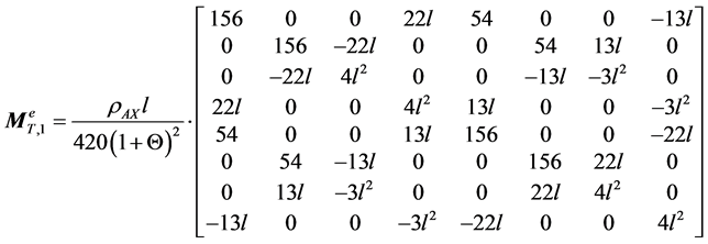
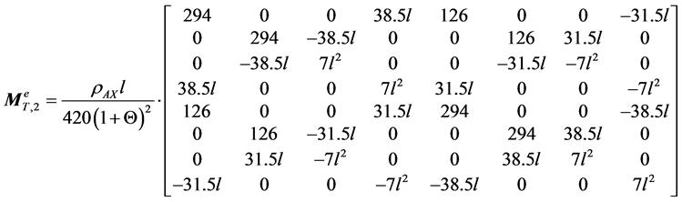
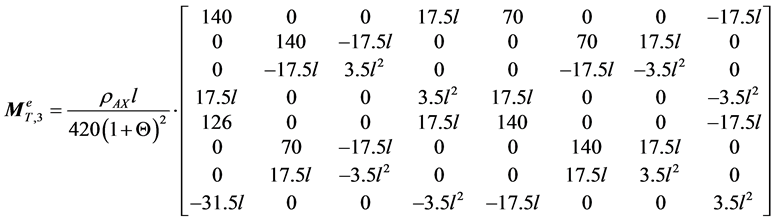
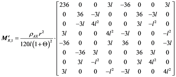
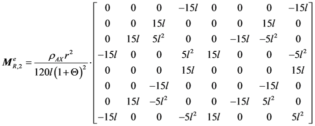
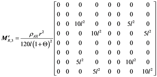
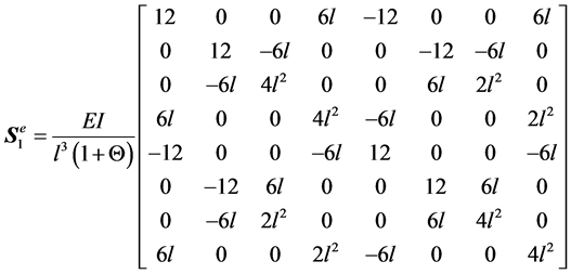
 are all determined based on the dimensions and material of the spindle shaft, and
the details of these matrices can be found in Appendix A, where the elements are
modeled as Timoshenko beams. Note that no structural damping or axial forces are
considered in the model.
are all determined based on the dimensions and material of the spindle shaft, and
the details of these matrices can be found in Appendix A, where the elements are
modeled as Timoshenko beams. Note that no structural damping or axial forces are
considered in the model.
The bearing stiffness matrix
 can be expressed by summing up the stiffness of all bearings as
 (3)
(3)
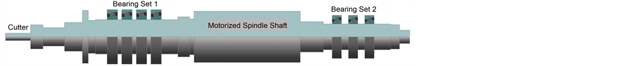
Figure 1. A general spindle-bearing system.
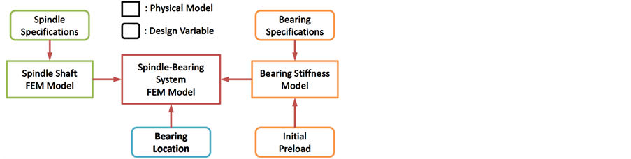
Figure 2. Mechanism of spindle-bearing system FEM model.
where
 is the total number of bearings in the system and
 , with the same size as
 , is the stiffness matrix contributed by bearing
 . Usually the points of application of the bearings
are arranged on the joint stations of spindle shaft FEM model [13] . If we neglect the axial stiffness contributed
by the bearing as in the analysis of the spindle shaft, the entries of
. Usually the points of application of the bearings
are arranged on the joint stations of spindle shaft FEM model [13] . If we neglect the axial stiffness contributed
by the bearing as in the analysis of the spindle shaft, the entries of
 can be written as
 (4)
(4)
where ,
,
 is the radial stiffness of bearing
 , and
, and
 is the joint station which the bearing is acted on. The static radial stiffness
 of an angular-contact ball bearing can be represented by the bearing stiffness equation
as a function of axial preload
of an angular-contact ball bearing can be represented by the bearing stiffness equation
as a function of axial preload , ball diameter
 , number of balls
 and contact angle
 [21] :
 (5)
(5)
where
 is an empirical data decided by the experimental results.
In order to find the natural frequencies of the system, we relate the vibration
problem to the generalized eigenvalue problem by substituting
 into Equation (1), which results in [13]
 (6)
(6)
 (7)
(7)
where
 is the system natural frequency,
 is the eigenvalue, and
 is the eigenvector.
To find a nonzero solution
 of Equation (6), we must have [22]
 (8)
(8)
which is the characteristic equation of , and the roots of which are the eigenvalues of
 . Expansion of Equation (8) by cofactors results
in a
. Expansion of Equation (8) by cofactors results
in a
 th-degree polynomial equation in
 , i.e. the eigenvalues of
 are
are , and therefore, the natural frequencies are
 ;
;
for each eigenvalue, there is a corresponding eigenvector.
3. Mathematical Model of the Bearing Location Optimization
In this research, we define the locations of bearings as the design variables. Assume
that there are
 sets of bearings to be installed on the spindle system, and for set
 ,
,
 identical bearings are used and, therefore,
 . Under this condition, the locations
of bearings of set
. Under this condition, the locations
of bearings of set
 can be represented as
 (9)
(9)
where the real number , named local design variable, indicates
the coordinate of the middle line of bearing
, named local design variable, indicates
the coordinate of the middle line of bearing
 of the bearing set
 . The lower the bearing sets numbered,
the closer their locations are to the original point. Since the bearings are identical
within a set, index
. The lower the bearing sets numbered,
the closer their locations are to the original point. Since the bearings are identical
within a set, index
 can also be used to represent the sequence of the bearings such that the bearings
with lower
can also be used to represent the sequence of the bearings such that the bearings
with lower ’s are closer to the original point. Therefore,
for bearing set
’s are closer to the original point. Therefore,
for bearing set ,
,
 and
and
 are the coordinates of the two end bearings respectively. The adjacent bearings
of bearing
are the coordinates of the two end bearings respectively. The adjacent bearings
of bearing
 are bearings
 and
and
 for
for . The locations of all bearings
 can be formed by assembling all
 as
as
 (10)
(10)
Besides the local variables, we define the global design variables as , which are utilized in calculating natural
frequencies after being converted into the corresponding numbers of joint stations
in FEM, and for a local variable owning an index
, which are utilized in calculating natural
frequencies after being converted into the corresponding numbers of joint stations
in FEM, and for a local variable owning an index , the index
 for its representing global variable can be evaluated by
 (11)
(11)
with .
.
Since the FMNF is the smallest among the natural frequencies of spindle-bearing systems, maximizing it draws the following objective function
 (12)
(12)
where . As discussed in Section 2,
 is the square root of eigenvalue
 and depends on
 since the matrix
 is a function of
 .
.
There are two different kinds of location-related constraints for the design variables considered in this research. First, the locations of bearings are ordinarily constrained by, for example, the geometrical boundaries of the segments where they are located. This kind of constraint is set to avoid interference with other parts, and or by the requirements originated from the results of other analyses such as statics. Here we name those constraints as Type I constraints and represent them with
 (13)
(13)
where
 and
and
 are the upper and lower limits of
 respectively.
The second type of constraints, Type II constraints, reflects the fact that the
least amount of spacing between two bearings must be greater than a specified value
such as the width of the bearing. Apparently, only the bearings within the same
group would be involved in the same constraint equations of Type II constraints.
If the smallest spacing of bearings
 and
and
 in the bearing set
 is recognized as
 , the constraints can be written as
 (14)
(14)
Ideally, the optimal solutions are obtained by identifying the ones possessing the maximum FMNF from the feasible solutions. However, since the objective function is complicated and nonlinear, it may be difficult or even impossible to derive an analytical or gradient-based method to solve the optimization problem. In this paper, a GA-based approach is constructed instead to search for the optimal solutions, which simultaneously satisfy all the constraints presented in Equation (13) and Equation (14).
4. Formulation of the Genetic Algorithm
As a randomized population-based search technique, GA utilizes genetic operators, i.e. crossover and mutation, inspired by natural evolution process to manipulate individuals in a population over generations to improve their fitness gradually based on the “survival of the fittest” strategies. The individuals in GA are likened to chromosomes which are most commonly represented as strings with an equal length of binary numbers formed by the coded design variables, and to each chromosome, there corresponds a value of the objective function, referred to as the fitness of the chromosome [23] .
To encode the real variables
 as binary numbers for forming the chromosome, we adopt the simple binary representation
scheme with
as binary numbers for forming the chromosome, we adopt the simple binary representation
scheme with
 bits [24] . The value of bit number
 is generally determined based on the required precision of the design variables.
For each component
is generally determined based on the required precision of the design variables.
For each component , by translating and scaling, we map its feasible
region
, by translating and scaling, we map its feasible
region
 onto the interval
 . The integers in the interval
 are then expressed as
 -bit binary strings
 , which defines the corresponding encoding
variable of
, which defines the corresponding encoding
variable of
 as
as
 (15)
(15)
where ,
,
 , and by collecting all
 ’s, we can form
 , the design variables in binary format.
As a result, the chromosome
, the design variables in binary format.
As a result, the chromosome
 can be constituted by attaching the
 -bit binary strings of all variables, end for end, in sequence
as
-bit binary strings of all variables, end for end, in sequence
as
 (16)
(16)
where
 is the length of chromosome
 .
.
 can be converted back to
 with a similar reverse transformation.
When we perform the decoding tasks to convert the binary codes back to real numbers, the feasible regions of variables must be identified deliberately according to the constraints applied to them. For a simple problem with fixed upper and lower limits, we can conduct decoding on all variables simultaneously since they are independent to each other. However, for mutually dependent variables such as those considered in this paper, their values in new generations, yielded by genetic operations of GA, may violate the dependency constraints (such as Type II constraints) if we try to decode the variables parallel in time or fail to handle the dependencies of the variables properly. There are several methods to ensure variable dependent constraints satisfied during GA optimization. The most effective approach is to restrict the search to valid regions of the search space, i.e. the chromosome is decoded in such a way that invalid solutions are prevented. We can thereby avoid wasting effort by evaluating infeasible solutions [25] .
In this research, to ascertain that the design variables satisfy all constraints
after decoding from binary codes to real values, we propose the Sequential Decoding
Process (SDP), in which the valid regions of variables are decided one by one, sequentially.
Since the locations of bearings of two different sets are independent, we can simultaneously
decode the variables within different bearing sets at the same time, and for each
set of bearings, we decode the variables, from the first to the last, in sequence.
The first step of SDP is converting the global binary variable
 to the local binary variable
 by using Equation (11). Then, for each bearing set
 ,
,
 , the binary
 , with respect to global
 , is decoded into real
 by using the standard binary decoding formula for
 from 1 to
 , in sequence:
 (17)
(17)
where if , the valid region
 ; if
; if , the valid region
 ; the values of
 ,
,
 , and
, and
 are specified in the constraints. After all
 are evaluated, we can obtain values of the global variables
 by the global-local transition equation as indicated in Equation (11).
Now that the above representation scheme has been defined, the procedure of applying the proposed SDP and GA, which is called SDP-GA, to search for the optimal solutions of the mathematical model is shown in Figure 3 and summarized as [26] :
1) Utilize a random number generator to create an initial population which consists
of
 individuals, each with an
 binary string.
2) Extract the values of variables for each individual by reading
 sets of
 binary digits and decoding into real numbers through the SDP. The fitness values,
FMNF, for all individuals are evaluated by solving Equation (8), where the locations
of bearings necessitate to be the joint stations of the finite element model, which
is coded and tested antecedently.
binary digits and decoding into real numbers through the SDP. The fitness values,
FMNF, for all individuals are evaluated by solving Equation (8), where the locations
of bearings necessitate to be the joint stations of the finite element model, which
is coded and tested antecedently.
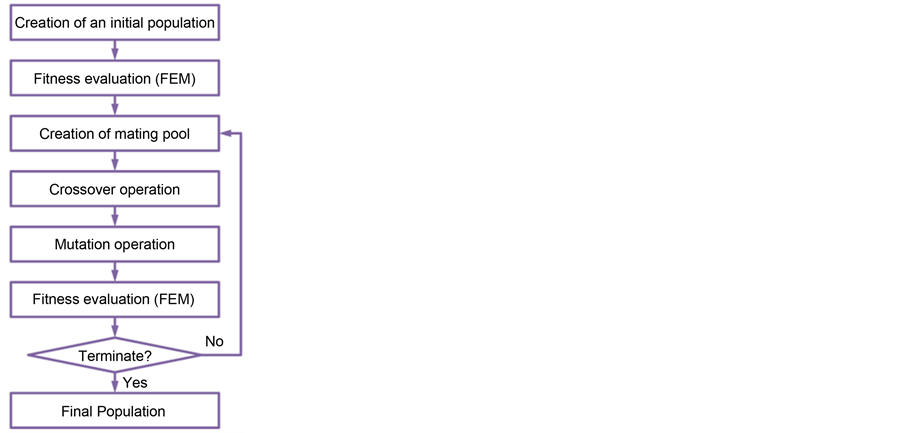
Figure 3. Flowchart of the SDP-GA.
3) Create a mating pool by using the proportional selection procedure, such as a
simulated roulette wheel, to choose the members in the initial population to form
a mating pool with a size , in which the chance of an individual being selected
for the mating pool is proportional to its fitness value.
, in which the chance of an individual being selected
for the mating pool is proportional to its fitness value.
4) Perform crossover operation on the mating parent pool to produce offspring. The
crossover operation adopted in this research involves randomly choosing two chromosomes
from the mating pool and an integer
 in the range of 1 to
 . The first
 positions of the parents are exchanged to produce two children.
5) Perform mutation operation by visiting every bit of all individuals of the new
population and switching the bit from 0 to 1 or 1 to 0 with a mutation probability .
.
6) Evaluate the population as what we did in step 2. The highest fitness value and the corresponding variable values are stored. A generation is now completed.
7) If the preset number of generations
 is complete, the process is stopped; otherwise, go to step 3.
Note that the size of population , the number of generations
 , and the mutation probability
 are generally decided with a few experiments to ensure a good convergence. However,
to further determine the optimal values of the parameters in this research, we conduct
statistical analysis such as design of experiments (DOE), analysis of variance (ANOVA),
and linear regression [27] .
are generally decided with a few experiments to ensure a good convergence. However,
to further determine the optimal values of the parameters in this research, we conduct
statistical analysis such as design of experiments (DOE), analysis of variance (ANOVA),
and linear regression [27] .
5. An Illustrative Example
To demonstrate the validity of the proposed SDP-GA, a real bearing location optimization problem of a high-speed spindle-bearing system design is exemplified in this section. It is assumed that the concept design stage has already been completed, and the results are summarized as specifications in Table 1 and Table 2 for the spindle shaft and bearings, respectively. The spindle shaft in this illustrative case is made of steel and constitutes 14 cylinders with different diameters. Table 1 shows the material properties of the spindle shaft, and the length and diameter of each segment as well as the number of elements that each segment is divided into in the FEM model. There are two different kinds of bearings, types ACB1 and ACB2, used in the example, and their specifications are indicated in Table2 The table also includes the widths of the bearings and the data required in Equation (5) for calculating their stiffnesses with the assumption that preloads applied on bearings are not affected by their locations. The results are also provided in the last column of the table.
If in the system level design stage, four bearings, two of type ACB1 on segment
7 and two of type ACB2 on 12, are planned to be installed in the system, i.e. ,
,
 , and
, and , we assign the global and
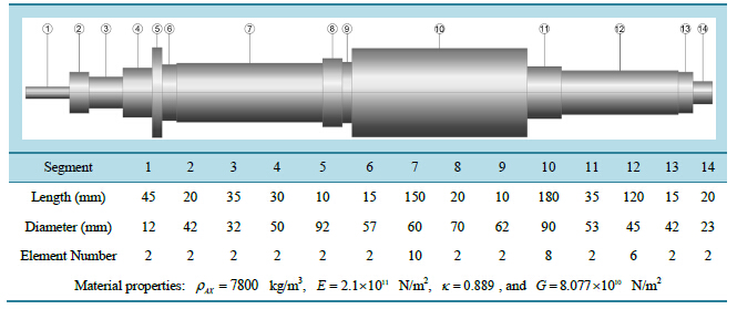
Table 1 . Dimensions and element numbers for the spindle shaft.
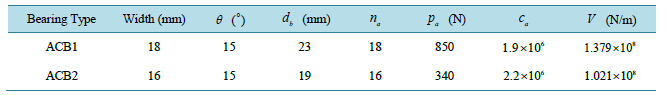
Table 2. The specifications of the bearings.
 and
and

where the set formed by the two bearings on segment 7 is numbered one and the set
on segment 12 is numbered two. Our objective is to maximize
 of the spindle system. The constraints of the design variables can be derived from
the data provided in Table 1 and
Table2 Assumed that geometry limits are the only sources of Type I constraints.
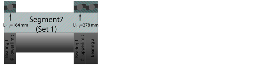
These constraints for the design variables are illustrated as
Figure 4. As revealed in Figure 4(a), for
example, the lower limit
of the spindle system. The constraints of the design variables can be derived from
the data provided in Table 1 and
Table2 Assumed that geometry limits are the only sources of Type I constraints.
These constraints for the design variables are illustrated as
Figure 4. As revealed in Figure 4(a), for
example, the lower limit
 of
of
 can be obtained by adding the left end coordinate of segment 7 and half of the width
of the type ACB1 bearing, i.e.
can be obtained by adding the left end coordinate of segment 7 and half of the width
of the type ACB1 bearing, i.e.
 mm. The upper limit
 is equal to subtracting the right end coordinate of segment 7 off 1.5 times of the
width of type ACB1 bearing, i.e.
is equal to subtracting the right end coordinate of segment 7 off 1.5 times of the
width of type ACB1 bearing, i.e.
 mm, where the origin point is located on the left end of the
spindle shaft. The type I constraints for the other three design variables can be
obtained in a similar way and the results are shown in
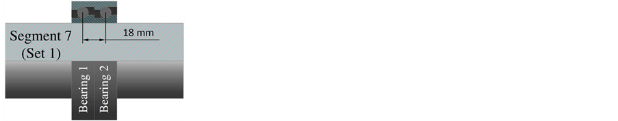
Figure 4. Type II constraints specify the least spacing between adjacent
bearing pairs. As shown in Figure 5, the least
distance between
mm, where the origin point is located on the left end of the
spindle shaft. The type I constraints for the other three design variables can be
obtained in a similar way and the results are shown in
Figure 4. Type II constraints specify the least spacing between adjacent
bearing pairs. As shown in Figure 5, the least
distance between
 and
and
 is the width of the bearing ACB1, which is equal to 18 mm, and between
 and
and
 is 16 mm, the width of bearing ACB2. Table 3 summarizes
all constraints for the four local design variables and also their valid regions
utilized in SDP-GA.
is 16 mm, the width of bearing ACB2. Table 3 summarizes
all constraints for the four local design variables and also their valid regions
utilized in SDP-GA.
Since there are only four variables in this case, we can reach the global optimal
solution as
 mm and the corresponding
 being 794.622 Hz by an exhaustive search with the precision as 0.5 mm. However,
even with only four variables, to obtain the results, the FMNF-related eigen-
being 794.622 Hz by an exhaustive search with the precision as 0.5 mm. However,
even with only four variables, to obtain the results, the FMNF-related eigen-
 (a)
(a)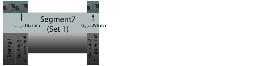 (b)
(b)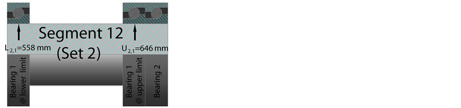 (c)
(c)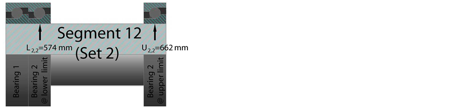 (d)
(d)
Figure 4.
Type I constraints for (a) ; (b)
; (b) ; (c)
; (c) ; and (d)
 .
.
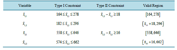
Table 3 . The constraint equations and valid regions of the design variables (all units are in mm).
 (a)
(a)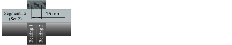 (b)
(b)
Figure 5. Type II constraints
for (a)
 and
and ; and (b)
 and
and .
.
value-solving subroutine has to be executed 414,855,255
 times, which takes about 240 days if one execution takes 0.05 seconds. To a design
project, 240 days may be too long to wait for a decision and the schedule is likely
to be delayed. To avoid such a tedious, exhaustive search, the alternative GA approach
provides a more efficient approach in obtaining an acceptable, near optimal solution.
times, which takes about 240 days if one execution takes 0.05 seconds. To a design
project, 240 days may be too long to wait for a decision and the schedule is likely
to be delayed. To avoid such a tedious, exhaustive search, the alternative GA approach
provides a more efficient approach in obtaining an acceptable, near optimal solution.
To code a computer program for searching for the optimal solutions by following
the SDP-GA procedures developed in Section 4, we need to decide bit numbers of the
design variables first. If the precision is required to be at least 0.5 mm and since
the largest interval for the design variables is 114 mm, the binary number , in order to guarantee the required precision,
must satisfy
, in order to guarantee the required precision,
must satisfy , which leads to
 , and such that the length of chromosome
 . Following the procedures indicated in
Figure 3, a computer program which constitutes
a main script M-file to execute the SDP-GA and a supporting function M-file to calculate
the FMNF, is coded in MATLAB. However, we still need to determine the parameters
. Following the procedures indicated in
Figure 3, a computer program which constitutes
a main script M-file to execute the SDP-GA and a supporting function M-file to calculate
the FMNF, is coded in MATLAB. However, we still need to determine the parameters ,
,
 , and
, and
 before running SDP-GA in searching for the optimal solutions.
In this paper, we use the statistics techniques DOE to identify the optimal values of the parameters under the practical assumption that the allowable time to decide the locations of bearings is one minute, i.e. the number of calculations for finding the eigenvalues must be 1200 at most if each eigenvalue evaluation takes 0.05 seconds.
As the total number of eigenvalue calculations
 in the SDP-GA optimization process, to satisfy the required calculation number 1200,
possible values of the parameters
in the SDP-GA optimization process, to satisfy the required calculation number 1200,
possible values of the parameters
 and
and
 can be expressed as
 combinations that include (16,74), (20,59), (30,39), and (40,29), where the smallest
 is set as 16 since it is the smallest number of chromosomes to prevent a population
from ending up with identical chromosomes. Because
is set as 16 since it is the smallest number of chromosomes to prevent a population
from ending up with identical chromosomes. Because
 and
and
 are dependent, we use the levels of
 to represent the combinations. The third parameter
 is typically very small [24] , therefore, the
possible values considered here are 0.005, 0.01, and 0.02.
is typically very small [24] , therefore, the
possible values considered here are 0.005, 0.01, and 0.02.
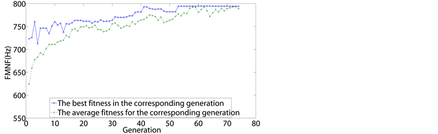
To examine convergence, Figure 6 shows the evolution
of the optimization process in a certain test run for all four candidates
 with
with
 respectively, where the maximum and average values of FMNF for each of the generations
are presented. From the figures, we can find that, as generations go by, not only
does the best chromosome of the population improve, but the rest in the entire population
also improve. This implies that the proposed SDP-GA approach not only provides a
single solution, but also a family of good-quality solutions.
respectively, where the maximum and average values of FMNF for each of the generations
are presented. From the figures, we can find that, as generations go by, not only
does the best chromosome of the population improve, but the rest in the entire population
also improve. This implies that the proposed SDP-GA approach not only provides a
single solution, but also a family of good-quality solutions.
After preliminarily confirming the convergence of the proposed SDP-GA algorithm,
to decide the levels for parameters
 and
and , a two-factor experiment is performed with FMNF as the response
variable and with
, a two-factor experiment is performed with FMNF as the response
variable and with
 and
and
 as the main factors. Since
 and
and
 are with 4 and 3 levels respectively, there are 12 different combinations or cells
of the two factors. In a complete balanced experimental design, we obtain 30 observations
(replication measurements) from each of the 12 cells. The sums, sums of squares,
averages, and standard deviations of the 30 observations for each cell are calculated
and shown in Table4 Based on the information provided
in Table 4, the ANOVA table for the two-factor
problem is shown in Table5 Under the level of significance
are with 4 and 3 levels respectively, there are 12 different combinations or cells
of the two factors. In a complete balanced experimental design, we obtain 30 observations
(replication measurements) from each of the 12 cells. The sums, sums of squares,
averages, and standard deviations of the 30 observations for each cell are calculated
and shown in Table4 Based on the information provided
in Table 4, the ANOVA table for the two-factor
problem is shown in Table5 Under the level of significance , since the
 -statistics of

 and of

 , we conclude that only the main effect
 affects FMNF. Furthermore, since the
 -statistic of interaction
 , there is no indication of interaction between
these two factors. The last column of Table 5 shows
that the
, there is no indication of interaction between
these two factors. The last column of Table 5 shows
that the
 -value for the test statistic for the main effect
 is considerably less than 0.05, while for the main effect
 and the interaction are greater than 0.05. A graph of the FMNF averages compared
to levels of
and the interaction are greater than 0.05. A graph of the FMNF averages compared
to levels of
 for each
 is shown in Figure 7. Notice that of the 12 experimental
configurations considered, the optimum configuration employs
is shown in Figure 7. Notice that of the 12 experimental
configurations considered, the optimum configuration employs
 at
at
 in the
 (a)
(a)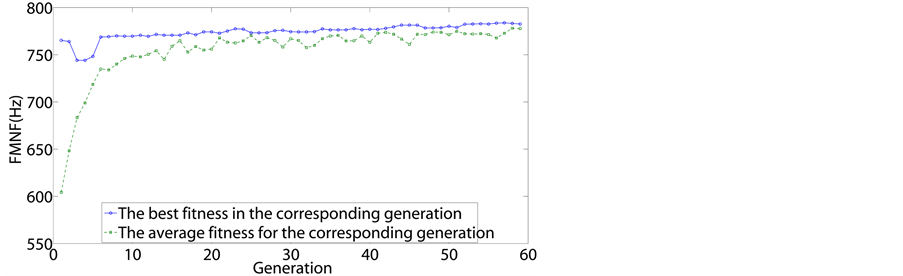 (b)
(b)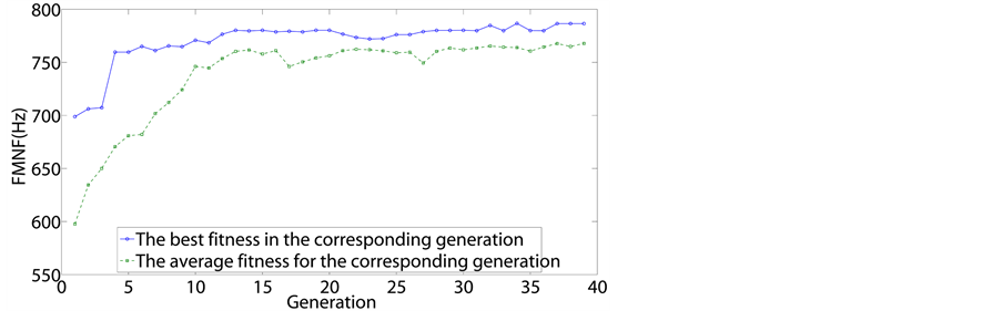 (c)
(c)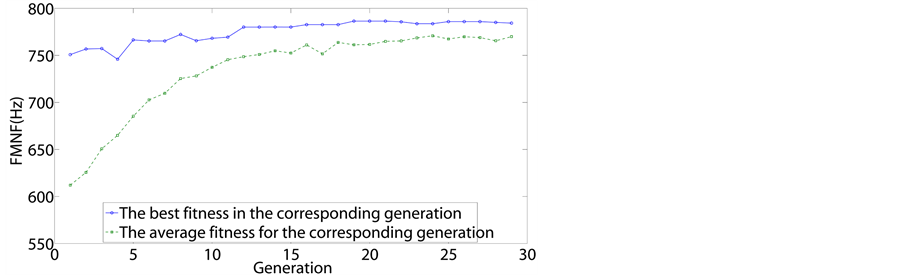 (d)
(d)
Figure 6. Results of a
certain test run for
 .
.
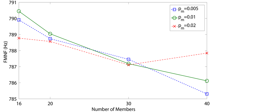
Figure 7. Graph of average
FMNF versus numbers of members for all values of .
.
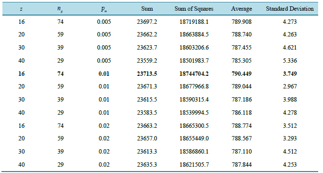
Table 4. Results of factorial design for parameters of SDP-GA.
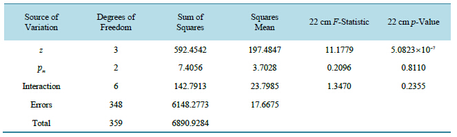
Table 5. The analysis of variance table for the FMNF data.
figure, where the average FMNF is about 790.449 Hz. In summary, under the requirement
that the optimal locations of bearings are obtained in one minute, after conducting
the two-factor factorial experiments and analysis of variation, the optimal parameters
of the GA are decided as
 (highlighted in Table 4), which can be applied
to determine the optimal locations of bearings not only for the original design
and the engineering changes, but also for the sensitivity studies of the design
parameters.
(highlighted in Table 4), which can be applied
to determine the optimal locations of bearings not only for the original design
and the engineering changes, but also for the sensitivity studies of the design
parameters.
In the 30 outcomes from the experiment of SDP-GA with optimal parameters , the best and worst ones are 794.625 Hz and
783.589 Hz, which compare to the results obtained by the exhaustive search, the
differences are about +0.000% and −388%, respectively. It is noticeable that
the best result is slightly better than that of exhaustive search (794.622 Hz) since
the precision of the former is finer than the later, and therefore, we replace the
value of
, the best and worst ones are 794.625 Hz and
783.589 Hz, which compare to the results obtained by the exhaustive search, the
differences are about +0.000% and −388%, respectively. It is noticeable that
the best result is slightly better than that of exhaustive search (794.622 Hz) since
the precision of the former is finer than the later, and therefore, we replace the
value of
 with 794.625 Hz. Table 6 summarizes the optimal
values of the four design variables, the corresponding FMNF's, and the final spindle-bearing
system drawings for the exhaustive search and the best and worst runs. Moreover,
since the average and standard deviation of FMNF for this combination are 790.449
Hz and 3.749 Hz respectively, the approximate 95% confidence interval on the mean
FMNF
with 794.625 Hz. Table 6 summarizes the optimal
values of the four design variables, the corresponding FMNF's, and the final spindle-bearing
system drawings for the exhaustive search and the best and worst runs. Moreover,
since the average and standard deviation of FMNF for this combination are 790.449
Hz and 3.749 Hz respectively, the approximate 95% confidence interval on the mean
FMNF
 is
is
 (18)
(18)
Therefore, if we can tolerate the potential errors of the SDP-GA approach as discussed
above and indicated in Table 6, the number of times
to run the subroutine for solving the eigenvalues can be reduced to 1200, which
is equal to
 of that the exhaustive search requires.
Apparently, the quality of the optimal solutions shall be better if we are allowed
to perform more calculations in the GA optimization. To investigate the influences
of calculating times on the results of SDP-GA by using the optimal parameter values
 and
and , as obtained in the above analysis, a series of 30-run tests
are conducted, with total eigenvalue calculating times
, as obtained in the above analysis, a series of 30-run tests
are conducted, with total eigenvalue calculating times , 6000, 18,000, and 30,000, which correspond to
 , 374, 1124, and 1874 respectively. The results
are summarized in Table 7, where the results of
, 374, 1124, and 1874 respectively. The results
are summarized in Table 7, where the results of

 are also included. From the table, we can find that as the
 increases, the average FMNF increases while the standard deviation decreases, which
confirms that the qualities of optimal solutions are improved with more iterations
by the SDP-GA. The maximum and minimum FMNF obtained in each
increases, the average FMNF increases while the standard deviation decreases, which
confirms that the qualities of optimal solutions are improved with more iterations
by the SDP-GA. The maximum and minimum FMNF obtained in each
 are also provided in the table, and they also perform better in larger
 . Finally, the last column of the table records
the numbers of outcomes hitting
. Finally, the last column of the table records
the numbers of outcomes hitting , where we can find that the frequencies are greater
with larger
, where we can find that the frequencies are greater
with larger , At
, At , this number even reaches 15, i.e. 50% of the
experimental runs hit
, this number even reaches 15, i.e. 50% of the
experimental runs hit . By using the extra information of sum and sum
of squares provided in Table 7, we can derive the
linear regression equation of FMNF vs
. By using the extra information of sum and sum
of squares provided in Table 7, we can derive the
linear regression equation of FMNF vs
 as [27]
 (19)
(19)
Equation (19) can be used to decide the number
 needed to reach a certain average value of FMNF. For example, if we want the results
with an average value 793 Hz, the required
needed to reach a certain average value of FMNF. For example, if we want the results
with an average value 793 Hz, the required
 can be calculated and rounded to an integer, as 1536, which is equal to 20.5 minutes
if each eigenvalue calculation takes 0.05 seconds, since
can be calculated and rounded to an integer, as 1536, which is equal to 20.5 minutes
if each eigenvalue calculation takes 0.05 seconds, since
 when
when![]() .
.
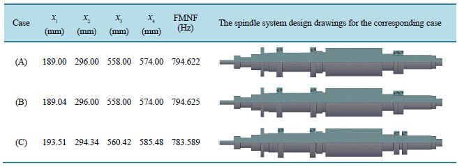
Table 6. The results for (A) The exhaustive search;
(B) The best run of ; and (C) The worst run of
 .
.
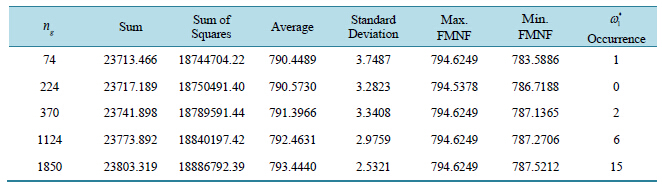
Table 7. Results of 30 runs for , 224, 370, 1124, and 1850.
6. Conclusion
This paper has developed a GA-based optimization approach to search for the optimal
locations of bearings installed on a spindle shaft to maximize the FMNF. First,
an FEM dynamic model of the spindle-bearing system is formulated, and by solving
the eigenvalue problem derived from the equations of motion, the natural frequencies
of the spindle system can be acquired. Next, the mathematical model is built, which
includes the objective function to maximize FMNF and the constraints to limit the
locations of the bearings with respect to the geometrical boundaries of the segments
they located and the spacings between adjacent bearings. A customized GA optimization
procedure, SDP-GA, is designed to accommodate the dependent characteristics of the
constraints in the mathematical model. To verify the proposed SDP-GA optimization
approach, a four-bearing installation optimization problem of a illustrative spindle
system is investigated. The results show that the SDPGA provides good convergence
for the optimization searching process. By applying DOE and ANOVA, the optimal values
of GA parameters are determined as![]() ,
,
 , and
, and , under the restriction that the number
of executing the eigenvalue calculation subroutine is 1200. The best and worst outcomes
for the optimal GA parameter are 794.625 Hz and 783.589 Hz, and for the best one,
the locations for the four bearings are
, under the restriction that the number
of executing the eigenvalue calculation subroutine is 1200. The best and worst outcomes
for the optimal GA parameter are 794.625 Hz and 783.589 Hz, and for the best one,
the locations for the four bearings are
 mm. Compared to the exhaustive search with a maximum FMNF as 794.622 Hz, the 95%
confidence interval of mean FMNF obtained by the SDP-GA with optimal parameter values
is
mm. Compared to the exhaustive search with a maximum FMNF as 794.622 Hz, the 95%
confidence interval of mean FMNF obtained by the SDP-GA with optimal parameter values
is
 Hz; however, the calculation time consumed by SDP-GA is about
 of that of the exhaustive search. A linear regression equation is also derived to
estimate necessary calculation efforts with respect to the specific quality of the
optimization solution. From the results of this illustrative example, we can conclude
that the proposed SDP-GA optimization approach is effective and efficient.
of that of the exhaustive search. A linear regression equation is also derived to
estimate necessary calculation efforts with respect to the specific quality of the
optimization solution. From the results of this illustrative example, we can conclude
that the proposed SDP-GA optimization approach is effective and efficient.
Acknowledgements
This study was supported by the National Science Council of Taiwan (grant number NSC 102-2221-E-035-048).
References
- Bossmann, B. and Tu, J. (2002) Conceptual Design of Machine Tool Interfaces for High-Speed Machining. Journal of Manufacturing Processes, 4, 16-27.
- Lin, C.-W. and Tu, J. (2007) Model-Based Design of Motorized Spindle Systems to Improve Dynamic Performance at High Speeds. Journal of Manufacturing Processes, 9, 94-108.
- Al-Shareef, K. and Brandon, J. (1990) On the Effects of Variations in the Design Parameters on the Dynamic Performance of Machine Tool Spindle-Bearing Systems. International Journal of Machine Tools and Manufacture, 30, 431-445.
- Kang, Y., Chang, Y.-P., Tsai, J.-W., Chen, S.-C. and Yang, L.-K. (2001) Integrated CAE Strategies for the Design of Machine Tool Spindle-Bearing Systems. Finite Elements in Analysis and Design, 37, 485-511.
- Li, H. and Shin, Y. (2004) Analysis of Bearing Configuration Effects on High Speed Spindles Using an Integrated Dynamic Thermomechanical Spindle Model. International Journal of Machine Tools and Manufacture, 44, 347-364.
- Maeda, O., Cao, Y. and Altintas, Y. (2005) Expert Spindle Design System. International Journal of Machine Tools and Manufacture, 45, 537-548.
- Altintas, Y. and Cao, Y. (2005) Virtual Design and Optimization of Machine Tool Spindles. CIRP Annual, 54, 379-382.
- Srinivasan, S., Maslen, E. and Barrett, L. (1997) Optimization of Bearing Locations for Rotor Systems with Magnetic Bearings. Journal of Engineering for Gas Turbines and Power, 119, 464-468.
- Nelson, H. and McVaugh, J. (1976) The Dynamics of Rotor-Bearing System Using Finite Elements. Journal of Engineering for Industry, Transactions of the ASME, 93, 593-600.
- Zorzi, E. and Nelson, H. (1977) Finite Element Simulation of Rotor-Bearing Systems with Internal Damping. Journal of Engineering for Power, Transactions of the ASME, 7, 71-76.
- Nelson, H. (1980) A Finite Rotating Shaft Element Using Timoshenko Beam Theory. Journal of Mechanical Design, Transactions of the ASME, 102, 793-803.
- Lantto, E. (1997) Finite Element Model for Elastic Rotating Shaft. ACTA Polytechnica Scandinavica, Electrical Engineering Series, 88, 1-73.
- Inman, D. (2008) Engineering Vibrations. Pearson Education, Inc., Upper Saddle River.
- Holland, J.H. (1975) Adaptation in Natural and Artificial Systems. University of Michigan Press, Ann Arbor.
- Rao, S.S. (2009) Engineering Optimization: Theory and Practice. John Wiley and Sons, Hoboken.
- Huang, M., Chen, K. and Fung, R. (2010) Comparison between Mathematical Modeling and Experimental Identification of a Spatial Slider-Crank Mechanism. Applied Mathematical Modelling, 34, 2059-2073.
- Fiandaca, G., Fraga, E. and Brandani, S. (2009) A Multi-Objective Genetic Algorithm for the Design of Pressure Swing Adsorption. Engineering Optimization, 41, 833-854.
- Gomes, H. and Silva, N. (2008) Some Comparisons for Damage Detection on Structures Using Genetic Algorithms and Modal Sensitivity Method. Applied Mathematical Modelling, 32, 2216-2232.
- Chakraborty, I., Kumar, V., Nair, S. and Tiwari, R. (2003) Rolling Element Bearing Design through Genetic Algorithms. Engineering Optimization, 35, 649-659.
- Lin, C.-W. (2001) High Speed Effects and Dynamic Analysis of Motorized Spindles for High Speed End Milling. Ph.D. Thesis, Purdue University, West Lafayette.
- Wardle, F., Lacey, S. and Poon, S. (1983) Dynamic and Static Characteristics of a Wide Speed Range Machine Tool Spindle. Precision Engineering, 5, 175-183.
- Zill, D., Wright, W. and Cullen, M. (2011) Advanced Engineering Mathematics. Jones & Bartlett Learning, Burlington.
- Pham, D. and Karaboga, D. (2000) Intelligent Optimisation Techniques, Genetic Algorithms, Tabu Search, Simulated Annealing and Neural Networks. Springer, New York.
- Chong, E. and Zak, S. (2008) An Introduction to Optimization. Wiley-Interscience, Hoboken.
- Zalzala, A. and Fleming, P. (1997) Genetic Algorithms in Engineering Systems. IET, London.
- Belegundu, A. and Chandrupatla, T. (1999) Optimization Concepts and Applications in Engineering. Prentice Hall, Upper Saddle River.
- Montgomery, D. and Runger, G. (2011) Applied Statistics and Probability for Engineers. Wiley, Hoboken.
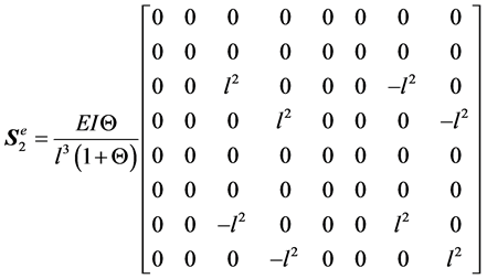
Appendix A
 (A.1)
(A.1)
where
 is the total element number, and the matrix
 is defined as:
 (A.2)
(A.2)
and for each element :
:
 (A.3)
(A.3)
 (A.4)
(A.4)
 (A.5)
(A.5)
 (A.6)
(A.6)
 (A.7)
(A.7)
 (A.8)
(A.8)
 (A.9)
(A.9)
 (A.10)
 (A.11)
 (A.12)
 (A.13)
 (A.14)
 (A.15)
 (A.16)
where
 is the axial mass density,
 is the length of the element,
 is the radius of the element,
 is Young’s modulus,
 is the moment of inertia,
 is the Timoshenko’s shear correction factor,
 is the cross-section area, and
 is the shear modulus of elasticity.