Applied Mathematics
Vol.5 No.4(2014), Article ID:43567,13 pages DOI:10.4236/am.2014.54058
Transfer of Global Measures of Dependence into Cumulative Local
Boyan Dimitrov1, Sahib Esa2, Nikolai Kolev3, Georgios Pitselis4
1Kettering University, Flint, USA
2Salahaddin University, Erbil, Iraq
3University of Sao Paulo, Sao Paulo, Brazil
4University of Piraeus, Piraeus, Greece
Email: bdimitro@kettering.edu, sahib_esa@yahoo.com, nkolev@ime.usp.br, pitselis@unipi.gr
Copyright © 2014 by authors and Scientific Research Publishing Inc.
This work is licensed under the Creative Commons Attribution International License (CC BY).
http://creativecommons.org/licenses/by/4.0/


Received 27 September 2013; revised 27 October 2013; accepted 5 November 2013
ABSTRACT
We explore an idea of transferring some classic measures of global dependence between random variables  into cumulative measures of dependence relative at any point
  in the sample space. It allows studying the behavior of these measures throughout the sample space, and better understanding and use of dependence. Some examples on popular copula distributions are also provided.
Keywords: Analysis of Variance; Copula; Correlation; Covariance; Multivariate Analysis; Measures of Dependence; Probability Modeling

1. Introduction
The ideas of transferring integral measure of dependence into local measures are probably not new. We got the clue from the works of [1] -[3] . Cooke raised the idea of the use of the indicator random variables (r.v.’s) in regression models to consider the regression coefficients as measures of local dependence. Genest [4] gave some more motivations on the need of transfer of overall (integrated) measures to the cumulative local functions. Dimitrov [2] revived some old measures of dependence between random events proposed by Obreshkov [5] , and noticed their convenience in the use of the studies of local dependence between r.v.s. [6] is an attempt looking at the cumulative dependence from the point of view of the so called Sibuya function, which is also used in studies of dependence.
We propose here a review of the classic statistical analysis approach, where the procedures are more or less routine to be used in the analysis of local dependence. The manuscript is built in the following way: Section 2 introduces the idea of the transfer in detail. Section 3 considers the covariance and correlation matrices between indicator functions for a finite family of random events. At this point it is worth noticing that the expressions for the entries  of the covariance matrix for identificators of random events
  coincide with the quantity
  introduced as connection between the events
  and
and  Similarly, the entries
  of the correlation matrix coincide with the expression called in [5] as correlation coefficient between the events
  and
and . Obreshkov approach is using different categories. Following these ideas, [2] exposes a relatively complete analysis of the two-dimensional dependence between random events, and establishes some more detailed properties of the Obreshkov measures of dependence. Similar expressions for the correlation between random events, are used in [4] . They call it correlation coefficient associated with pairs of dichotomous random variables. Long before [7] , p.311 uses correlation coefficient between indicator functions of two events, but does not elaborate any details.
Let  and
and  be two
  -sub-algebras of
 . The survey of [3] proposes the measure
 (1.1)
(1.1)
to be used as magnitude of dependence between  and
and . This measure is used for studying properties of a sequence
  of r.v.’s, when choosing
  and
and  generated by two remote members—
 and
and  of the sequence. The
  is called mixing. The similarity with the Obreshkov’s connection measure between events is obvious. However, this measure of dependence
  is a global measure limited within the interval
 , and does not have clear meaning of magnitude. Some of its properties are summarized in the statements of Section 3. Section 4 extends these results as integrated local measures of dependence between finite sequence of r.v.’s. Explicit presentations in terms of joint and marginal cumulative distribution functions (c.d.f.’s) are obtained. Some invariant properties are established in Section 5; Examples (explicit analytic and graphic) with popular copula distributions, and a bivariate Poisson distribution with dependent components illustrate these properties. 3-d surfaces with level curves consisting of points with constant cumulative magnitude of local dependence (covariance or correlation magnitude) in the sample space are drawn (Sections 5, 6, and 7).
2. The Idea for Measure Transfer
Let  be random variables (r.v.’s) defined on a probability space
  with joint cumulative distribution function (c.d.f.)

and marginals

Most of the conventional measures of dependence between r.v.’s used in the practice are integral (global). Usually they have the form of expected values of some specifically selected function . Sometimes
  can be a real number, a vector, or a matrix. The dependence measure “of type
 ” is expressed by the equation

Let  be a finite set of random events in the sample space
  of an experiment, where the r.v.’s
  are defined. Introduce the indicator r.v.’s

Then the domain of the r.v.’s  is a subset of the sample space
  of the r.v.’s
Definition 1. The quantity

is called measure of dependence of the type  between the random events
 .
.
Assume, the measure of dependence of type  is introduced, and its properties are well established and understood. For any choice of the point
  define the random events
 (1.2)
(1.2)
Obviously,  define the marginal distribution functions of the r.v.’s
 . Put these events in Definition 1, and get naturally the next:
Definition 2. The quantities

are called cumulative local measure of dependence of type  between the r.v.’s
  at the point
 .
.
As an illustration of the above idea we consider the frequently used and well known integral measures within a finite sequence of r.v.’s, the covariance and correlation matrices.
3. Covariance and Correlation between Random Events
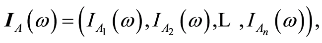
Introduce vector-matrices  and
and , and their transposed
  and
and . The covariance matrix between r.v.’s
  is
is
 (1.3)
(1.3)
By implementing the idea of the previous section, we introduce Covariance matrix between random events .
.
First, observe that  and
and

Introduce vectors
and

Formally, the covariance matrix  between the random events
  is defined by

Its entries are
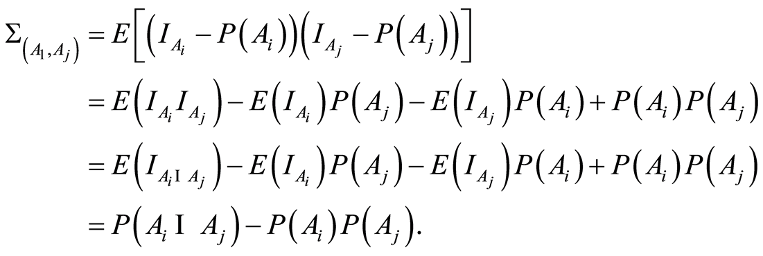 (1.4)
(1.4)
On the main diagonal of the covariance matrix  we recognize the entries
 (1.5)
(1.5)
where  is the complement event to the event
 . By making use of the standard approach we introduce the correlation matrix between random events

whose entries are the correlation coefficients between the indicators of respective events. Based on (1.4) and (1.5) for , they have the form
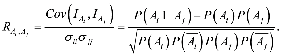 (1.6)
(1.6)
We call these entries correlation coefficients between random events  and
and . As one should expect, the entries on main diagonal are equal to 1. Each entry of the correlation matrix for
 , satisfies the inequalities
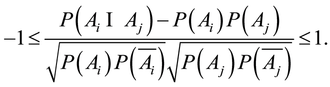 (1.7)
(1.7)
Let us focus on some basic properties of the entries of covariance and correlation matrices. They reveal also the information contained in terms of these matrices. Details can be seen in [2] .
Theorem 1. a) The covariance  and the correlation coefficient
  between events
  and
and 
equal 0 if and only if  and
and  are independent. The case includes the situation when one of the events
  or
or  is the sure, or the impossible event (then the two events also are independent);
b)  if and only if events
  and
and  coincide;
c)  if and only if events
  and
and  coincide (or equivalently, if and only if the events
  and
and  coincide);
d) The covariances between events  and
and  satisfy the inequalities
 (1.8)
(1.8)
The equalities in the middle of (0.8) hold only if the two events  and
and  obey the hypotheses stated in parts a), b) and c);
e) The covariance and the correlation coefficients between the events  and
and  and their complements
  and
and  are related by the equalities

and

The advantage of the considered measures is that they are completely determined by the individual (marginal) probabilities  of the random events, and by their joint probabilities
  An interesting fact is that we do not need the joint probability to calculate conditional probabilities between the events. If either of the measures of dependence
  or
or  is known then the the conditional probability
  can be found when marginal probabilities
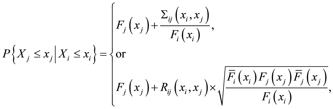
 are known. It holds Theorem 2. Given the measures
  or
or  and marginal probabilities
 , the conditional probabilities of one event, given the other, can be calculated by the equations
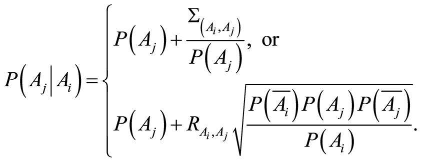 (1.9)
(1.9)
Remark 1. If the covariance, or the correlation between two events  and
and  is positive, the conditional probability of one event, given the other one, increases, compare to its unconditional probability, i.e.
  and the exact quantity of increase equals to
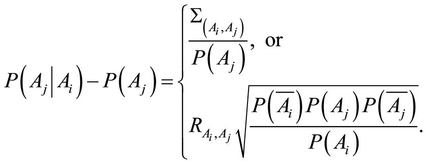 (1.10)
Conversely, if the correlation coefficient is negative, the information that one of the events has occurred, the chances that the other one occurs decrease. The net amount of decrease in probability is also given by (1.10).
4. Covariance and Correlation Functions Describe Cumulative Local Dependence for Random Variables
Here we continue developing the idea of Section 2 to illustrate how the cumulative local measures of dependence between r.v.’s are obtained and expressed in terms of the conventional probability distribution functions. Let  be arbitrary finite sequence of r.v.’s. For any choice of the real numbers
 , let
, let  be the random events as defined in (1)
  The covariance and correlation matrices for random events
  immediately turn into respective integrated measures of local dependence between the r.v.’s
  at the selected point
 . We discuss these matrices here, and focus on their specific forms in terms of the respective distribution functions. The covariance matrix function

whose entries are defined for any pair 
 by the equations
 (1.11)
represents the cumulative local covariance structure between r.v.’s  at the point
 . Analogously, we obtain the correlation matrix function

whose entries according to Equation (1.6), are
 (1.12)
Obviously, these matrices are functions of the joint c.d.f.’s  and of the marginals
 of the participating r.v.’s. The properties of these entries are described by Theorem 1, and Theorem 2. We notice here the following particular and important facts.
Theorem 3. a) The equality

holds if and only if the two events , and
, and  are independent at the point
 ;
;
b) The equality

holds if and only if the two events , and
, and  coincide at the point
 ;
;
c) The equality

holds if and only if the two events , and the complement
  coincide at the point
 . Then also the events
 , and
, and  coincide.
d) Given the dependence function measures  or
or  and marginal c.d.f.’s
 , the conditional probabilities
  and
and  can be evaluated by the expressions
and
Proof. The statement is just an illustration of the transfer of the results of Theorems 1 and 2 from random events to the case of events depending on parameters. We omit details.
Theorem 3 d) provides the opportunity to make predictions for either of the events , or
, or , given that the other event occurs, or does not occur. The absolute values of the increase (or decrease) of the chances of the r.v.
  to get values less than a number
  under conditions of known values of the variable
  compare to these chances without conditions, can be evaluated as shown in Remark 1. The evaluation is expressed in terms of the local measures of dependence and the marginal c.d.f.’d of participating r.v.’s.
Remark 4. [8] introduces positive quadrant dependence between two r.v.’s by the requirement: for all  to be fulfilled
  This is equivalent to the validity of
  everywhere. The reverse inequality, when it remains true for all
  Nelsen calls as negative quadrant dependence. Also there ([8] p. 189) the author gives some discussion about Local Positive (and Local Negative) Quadrant Dependencies between r.v.’s
  and
and  at a point
 , and does not go any further in its possible use. We are confident, that having local measure of dependence at a point, and especially, the measure of its magnitude given by the correlations functions
  offers the opportunity to use more. Namely, it is possible to classify the points in the plane according to their magnitude of dependence. For instance, there might be points of marginal independence, where the covariance equals zero. There can be areas of positive and negative dependence, depending on the sign of the covariance. There can be curves of constant cumulative correlations, e.g. curves given by the equations, like
  or
or , etc. Our examples below provide effective proofs of such facts.
5. Monotone Transformations of the Random Variables and Related Dependence Functions. Copula
Here we study how the dependence functions behave under increasing or decreasing transformations. Before we move on, we introduce the following notations in order to make exposition clearer. We will use the notations  and
and  for the covariance and correlation matrices of the random variables
  where
where  are arbitrary functions defined on the range of the arguments
 . Also we introduce notations
  and
and  to mark the variables for which the respective dependence functions are pertained.
Now we present the results with the following statement:
Theorem 4. Given arbitrary continuous functions  on the supports of the continuous r.v.’s
  and
and  respectively, such that
  and
and  do exist, we have:
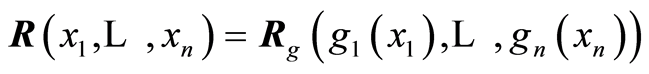
If  and
and  are all increasing functions, or if
  are all decreasing functions, then the values of the respective covariance and correlation functions at the respective points are related by the equations

and

Also the relations

and
are valid.
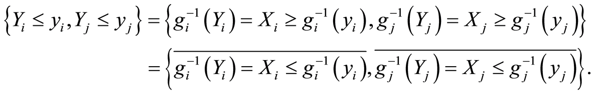
Proof. The statement follows from the fact that the following equivalence between the random events at any point  are valid:
If  and
and  are both increasing functions, then the following random events are equivalent
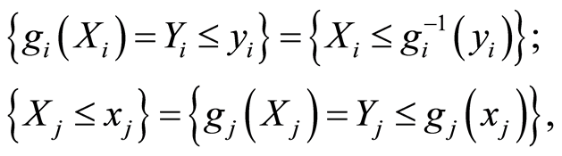
and equivalent are also the events

for all .
.
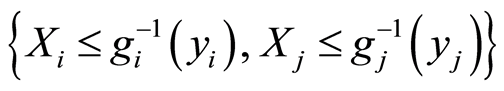
If  and
and  are both decreasing functions, then the following random events are equivalent
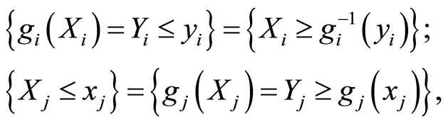
and also equivalent are
for all .
.
Next, we use the facts that the covariance and correlation matrix functions introduced in (1.11) and (1.12) for pairs of random events  and
and  are the same for any pairs of equivalent events
 , as well as for the pair of their complements
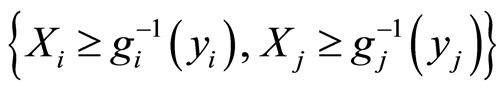 , according to Lemma 2 part b) are equal. The reason is that the respective probabilities used in the definition of the matrix entries of equivalent events also are equal.
Assume now, that  are continuous r.v.’s, and
  is their continuous distribution function, as well as its all marginals are. According to [8] , there exists unique n-dimensional copula
  (a n-dimensional distribution on the n-dimensional hyper-cube
  with uniform 1-dimensional marginals and any 2- and higher-dimensional marginals also being copulas) associated with
 , such that it is true
 (1.13)
Then it is true also
 (1.14)
Denote by  and by
  the covariance and the correlation matrix functions corresponding to the uniformly distributed on
  r.v.’s
  whose joint distribution function is the copula
 . We introduce the notations
  and
and  for the covariance and correlation matrix functions corresponding to the original r.v.’s
 .
.
The following statement holds:
Theorem 5. If  is a continuous
  -dimensional distribution function and
  is its associated copula, then the following relationships are true
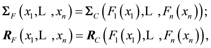
and also
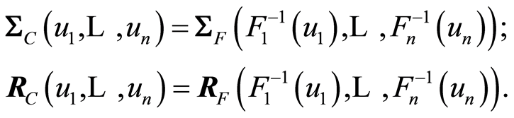
Proof. The proof of these relationships is a simple consequence from Theorem 4, when we notice that the copula is just the distribution of a set of random variables, obtained after a monotonically increasing transformation  or
or  is applied to each component of the original random vector
 , or to the vector
Both theorems explain how after transformation the local cumulative dependence structure for the new variables is transfered to the points related with the same transformations at each coordinate of the other set of random variables. The fact of curiosity is that the relationships in Theorem 5 completely repeats the relationships (1.13) and (1.14) which define the copula.
The next examples illustrate the covariance and correlation functions for two popular multivariate copula, which we borrow from [8] .
Examples
1) Farlie-Gumbel-Morgenstern (FGM) n-copula
The FGM n-copula is given by the equation
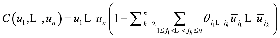
where the coefficients  and
and 
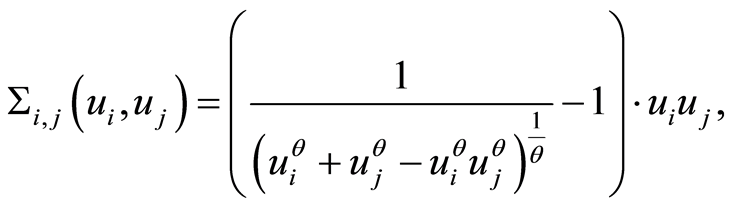
The entries of the covariance and the correlation matrices are respectively

and

We observe here, that the covariance and correlation functions keep constantly the sign of the parameter .
.
Moreover, the correlation functions  do not exceed the numbers
  for all
 .
.
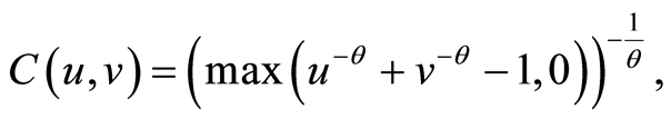
2) Clayton Multivariate Archimedean copula
The copula is given for any , by the equation

where  and the parameter
  For negative values of
  the maximum of the expression in the brackets and 0 must be taken, and
  must be fulfilled. For instance, if
  we should have
 .
.
The entries of the covariance and the correlation matrices in case of positive , are respectively
and

6. Maps for Dependence Structures on the Sample Space
A thorough analysis of the results in previous sections leads to an interesting opportunity to divide the sample space for any pair of r.v.’s  into areas of positive, or negative dependence between the events
  and
and . For this purpose, one can use the following curves:
Curve of Independence,  the set of all points
  in
in  where the correlation function
 . In other words,

Here the events  and
and  are independent for all points
  .
.
Curve of Positive Complete Dependence,  the set of all points
 , where the correlation function
 . In other words,

Here the events  and
and  coincide for all points
  .
.
Curve of Negative Complete Dependence,  the set of all points
 , where the correlation function
 . In other words,

Here either of the events  and
and  is equivalent to the complement of the other one for all points
 .
.
Additional mapping can be drown by making use of the Correlation Level Curves at level 

At each point of such a curve , the correlation function
  between the events
  and
and  equals to
 . and
. and .
.
When  is positive, the random variables
  are positively associated at the points
 . When
  is negative, the random variables
  are negatively associated ate the points
 .
.
In particular applications such curves may have important impact on understanding the dependence structure between the random variables . By the way, some of these curves may happen to be empty sets.
One can ilustrate these curves in the next examples, using 3-d plots of the surfaces  and
and  with the level curves. In our plots we have used the program system Maple, and graph just the correlation function.
Examples
Here we illustrate the information one may visually get from the mapping of the 3-d graphs for the considered above copula. We plot their correlation function  with
with . Since the pictures are the same for any pair of indices
 , we use notations without any indices.
1) The correlation functions for FGM copula (continued)
The two-dimensional marginal distributions of the multivariate FGM copula are given by one and the same equation, and we drop the subscripts:
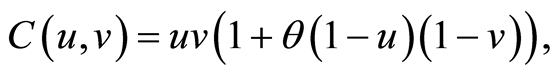
where 
The correlation function is respectively
and satisfies the inequalities  On Figure 1 we see the 3-dimensional graph of the surface
 , for the cases
  and
and .
.
2) Clayton Archimedean copula (continued)
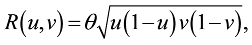
The two-dimensional marginal distributions of the multivariate Clayton copula also are given by the same equations, and we drop the subscripts:
The copula is given by the equation
and in the multivariate case it is required that  However the Clayton copula in the two-dimensional case is defined for all
  and
and 
The respective correlation function is
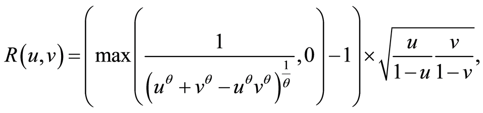
and this relation is valid for all .
.
To have a base for comparison (with the pictures in [8] p. 120, Figure 4.2), we consider the case , and present several level curves on the 3-d graph of
  Actually, the level curves
  are visible on the surface from which we see that
  is between 0 and 1.0. Results are pictured of Figure 2.
The 3-d graphs for this particular measure shown on Figure 2(b) of dependence between the two components of the copula closely imitate the situations given in the scatter-plots in the reference book [8] , but are more impressive and information giving.
Together with the surface plots, the correlation function and its level curves are quite more informative than the simulated scatter-plots used in copula.
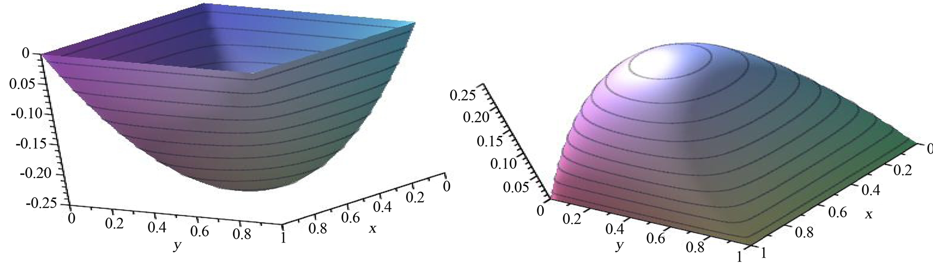 (a) (b)
Figure 1. Correlation function for the Farlie-Gumbel-Morgenstern copula with level curves, θ = ±1. (a) FGM-copula correlation function surface, θ = −1; (b) FGM copula correlation function surface, θ = 1.
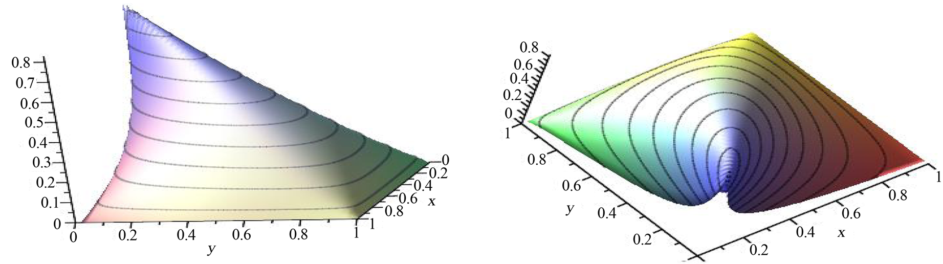 (a) (b)
Figure 2. Correlation function for the Clayton copula, θ = 4. (a) Clayton copula correlation function surface-a look from (1,1) corner; (b) Clayton copula correlation function surface-a look from (9,0) corner.
7. On the Use of the New Measures
At this point we believe that the introduced local measures of dependence can be used in similar ways as the covariance and correlation matrices are used in the multivariate analysis. However, because we think that the ideas developed here are so natural and simple, there will be no wonder if what we propose here is already in use. But, with the best of our knowledge, we have never seen anything similar, and we dare to say it under the risk we are not the first who offers such approach.
The results of Section 3 for random events may suit analysis of non-numerical, categorical, and finite discrete cases of random data similar to the ways as the numeric data are treated.
The results of Section 4 show that we are getting an opportunity to treat mixed discrete and continuous variables equally, using the cumulative distribution functions (marginal, and the two-dimensional).
If one treats the induces  of the events
  as time variables (time is
 ), the above approach may offer interesting applications in the areas of Time Series Analysis, as well as in the studies of sequences of random variables.
Obtained results may have impact on various side effect questions, and we leave it for other’s comments. We insist on main practical orientation of our results-same and similar as everything else build on the use of the covariance and correlation matrices in the multivariate analysis.
8. Further Expansion of the Idea of Transforming Measures
In addition, the new measures may be used in studying the local structures of dependence within rectangular areas of the sample spaces when the sets of random events are defined as type of Cartesian products

and by making use of the main idea of the transfer from the Introduction.
Another extension that may allow the involvement of the probability density functions (p.d.f.) could be obtained as in Section 4, by considering the elementary events

whose probabilities are
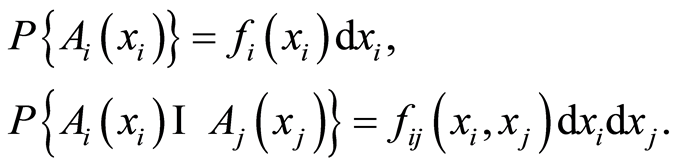
Here 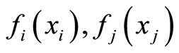 and
and  are the marginal and the joint probability densities of the r.v.’s
and of the pair  Since the densities do not have meaning of probabilities, for now we cannot use them in similar constructions. However, the picture changes in case of discrete variables.
As an illustration of this approach in the study of local dependence structure we consider the discrete case. The r.v.’s  and
and  have joint distribution
  and marginals
  and
and 
 Then the covariance function
  is defined by the equalities

The respective correlation function will be defined by
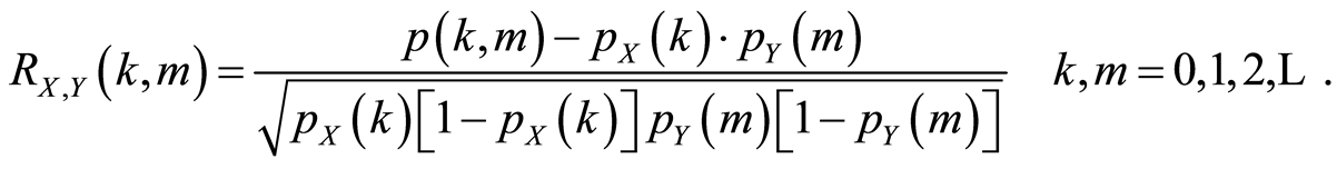
Graphing these functions, one can see the local dependence structure between the two variables at any point  and to evaluate its magnitude, and in addition will see the entire picture of this mutual dependence in the field-the range of the pair
As an illustration of this suggestion we consider the simplest Bivariate Poisson distribution constructed in the following way, borrowed from [9] . There are three Poisson distributed r.v.’s  of parameters
 Then it is supposed
 The dependence between
  and
and  comes from the involvement of
  in both components. Their marginal distributions are Poisson with parameters
  and
and  correspondingly. The joint distribution is given by

After substitution of this form of the joint distribution and the marginal Poisson distributions in the above expressions, we get the covariance and correlation functions and the study of the local dependence can start. We omit detailed analytical expressions for these functions which is not a problem to get but are too cumbersome to write here.
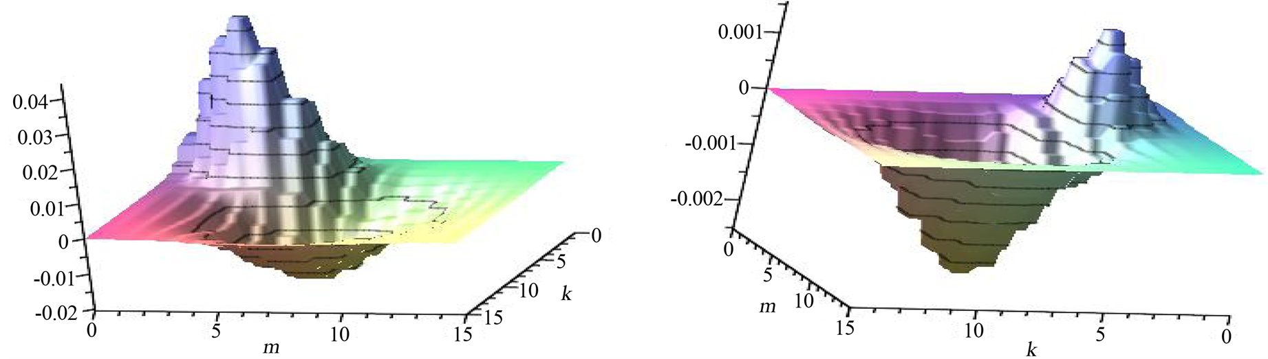
On Figure 3 we give an illustration of these functions by their 3-d graphs in the case when 
 and
and  The magnitude of dependence is not strong (the local correlation coefficient is too small). However, we observe that on the square
  the association is positive, when on the rectangle
  this dependence is negative and also is a bit stronger. Outside these areas the two variables are almost independent.
More exotic spots of dependences can be obtained when in Definition 2 the events  are chosen as

where  are any Borel sets on the real line, with
In our opinion, there is a number of follow up questions in the multivariate dependence analysis, and more illustrations on real statistical data will trace the utility of the offered approach.
9. Conclusions
In this paper we discuss the possibility to transfer conventional global measures of dependence onto measures of
 (a) (b)
Figure 3. Surfaces explain local dependence structure in the Bivariate Poisson distribution. (a) Dependent PoissonCovariance function; (b) Dependent Poisson-Correlation function.
dependence between random events, and then using another transfer to turn them into cumulative local measures of dependence between random variables.
We illustrate the method on the example of covariance and correlation matrices between random variables. Important results can be found in the discussion on some specific properties of the new measures, and in the qualitative information that may be derived from the meaning of these measures.
The behavior of these measures under monotonic transformations is established. It shows full coincidence between the pictures in the sample space of the original random variables and their respective copulas.
We found that locally the random variables may have areas of positive dependence and areas of negative dependence, as well as areas of local independence. This seems something interesting from informational point of view compared to the global measures of dependence.
Our suggestion is that the local measures of dependence offer important topological pictures to study. Our examples illustrate the new opportunities in this field.
Acknowledgements
The authors acknowledge FAPESP (Grant 06/60952-1, and Grant 03/10105-2), which gathered us for several days, where we had the opportunity to start the work on this exciting topic. We are thankful to Professor Roger Cook for his then unexpected spontaneous support during the Third Brazilian Conference on Statistical Modeling in Insurance and Finance, Maresias, Brazil.
References
- Cooke, R.M., Morales, O. and Kurowitcka, D. (2007) Vine in Overview. Proceedings of 3rd Brazilian Conference on Statist. Modeling in Insurance and Finance, 26-30 March 2007, 2-20.
- Dimitrovm B. (2010) Some Obreshkov Measures of Dependence and Their Use. Compte Rendus de l’Academie Bulgare des Sciences, 63, 15-18.
- Bradley, R.C. (2005) Basic Properties of Strong Mixing Conditions. A Survey and Some Open Questions. Probability Surveys, 2, 107-104.
- Genest, C. and Boies, J. (2003) Testing Dependence with Kendall Plots. The American Statistician, 44, 275-284. http://dx.doi.org/10.1198/0003130032431
- Obreshkov, N. (1963) Probability Theory. Nauka i Izkustvo, Sofia (in Bulgarian).
- Dimitrov, B., Kolev, N. and Goncalves, M. (2007) Some Measures of Dependence between Two Random Variables. Work Paper.
- Renyi, A. (1969) Foundations of Probability Theory. Holden-Day, San Francisco.
- Nelsen, R. (1999) An Introduction to Copulas. Springer, New York. http://dx.doi.org/10.1007/978-1-4757-3076-0
- Kocherlakota, S. (1988) On the Compounded Bivariate Poisson Distribution: A Unified Treatment. Annals of the Institute of Statistical Mathematics, 49, 61-70. http://dx.doi.org/10.1007/BF00053955