Applied Mathematics
Vol.4 No.8(2013), Article ID:35142,10 pages DOI:10.4236/am.2013.48151
Analysis of Stochastic Reliability Characteristics of a Repairable 2-out-of-3 System with Minimal Repair at Failure
1Department of Mathematical Sciences, Bayero University, Kano, Nigeria
2Department of Physics, Bayero University, Kano, Nigeria
Email: *Ibrahimyusuffagge@gmail.com, FatimaSK2775@gmail.com
Copyright © 2013 Ibrahim Yusuf, Fatima Salman Koki. This is an open access article distributed under the Creative Commons Attribution License, which permits unrestricted use, distribution, and reproduction in any medium, provided the original work is properly cited.
Received May 18, 2013; revised June 18, 2013; accepted June 25, 2013
Keywords: Minimal Repair; Reliability; Availability
ABSTRACT
In this paper, we study the reliability and availability characteristics of a repairable 2-out-of-3 system. Failure and repair times are assumed exponential. The explicit expressions of reliability and availability characteristics such as mean time to system failure (MTSF), steady-state availability, busy period and profit function are derived using Kolmogorov’s forward equations method. Various cases are analyzed graphically to investigate the impact of system parameters on MTSF, availability, busy period and profit function.
1. Introduction
During operation, the strengths of systems are gradually deteriorated, until some point of deterioration failure, or other types of failures. Maintenance policies are vital in the analysis of deterioration and deteriorating systems as they help in improving reliability and availability of the systems. Maintenance models assume perfect repair (as good as new), minimal repair (as bad as old) and imperfect repair which between perfect and minimal repair. There are systems of three/four units in which two/three units are sufficient to perform the entire function of the system. Examples of such systems are 2-out-of-3, 2-outof-4, or 3-out-of-4 redundant systems. These systems have wide application in the real world especially in industries. Many research results have been reported on reliability of 2-out-of-3 redundant systems. For example, [1] analyzed reliability models for 2-out-of-3 redundant system subject to conditional arrival time of the server. Reference [2] presented reliability and economic analysis of 2-out-of-3 redundant system with priority to repair, [3] studied MTSF and cost effectiveness of 2-out-of-3 cold standby system with probability of repair and inspection while [4] examined the cost benefit analysis of series systems with cold standby components and repairable service station. Reference [5,6] examined the cost analysis of two unit cold standby system involving preventive maintenance respectively. Reference [7] studied the cost and probabilistic analysis of series system with mixed standby components, and [8] studied cost benefit analysis of series systems with warm standby components involving general repair time where the server is not subject to breakdowns. The failure time and repair time are assumed to have exponential distribution. Measures of system effectiveness such MTSF, steady-state availability, busy period and profit function are obtained. Reference [9] studied availability of a system with different repair options, while [10] evaluate the reliability of network flows with stochastic capacity and cost constraint.
In this paper, a 2-out-of-3 redundant system is constructed and derived its corresponding mathematical models. The main contribution of this paper is two fold. First, is to develop the explicit expressions for MTSF, system availability, busy period and profit function. The second is to perform a parametric investigation of various system parameters on MTSF, system availability and profit function and capture their effect on MTSF, availability, busy period and profit function.
The rest of the paper is organized as follows. Section 2 the notations, assumptions of the study, and the states of the system. Section 3 gives the states of the system. Section 4 deals with models formulation. The results of our numerical simulations are presented and discussed in Section 5. The paper is concluded in Section 6.
2. Notations and Assumptions
2.1. Notations
 : Minimal repair rate of
 .
.
 : Failure rate of
 .
.
 : Rate of going into reduced capacity of
 .
.
 : Exchange rate of unit
  and
and  in reduced capacity simultaneously.
 : Minimal repair rate of unit
  and
and  simultaneously.
 : Failure rate of unit
  and
and  simultaneously.
 : Unit in full operation/reduced capacity/ failure/ standby.
2.2. Assumptions
1) The system is 2-out-of-3 system.
2) The system work in a reduced capacity before failure.
3) The systems have three states: normal, reduced and failure.
4) Unit failure and repair rates are constant.
5) Repair is as bad as old (minimal).
6) failure and repair time are assumed exponential.
7) The system failed when two units have failed.
8) The system is under the attention of two repairmen.
3. States of the System
3.1. Up States
 ,
,  ,
,
 ,
,  ,
,
 ,
, .
.
3.2. Down State
 .
.
4. Models Formulation
4.1. Mean Time to System Failure for System
Let  be the probability row vector at time
 , then the initial conditions for this problem are as follows:
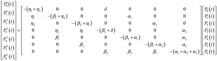
 we obtain the following system of differential equations:
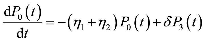
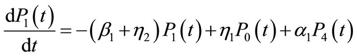
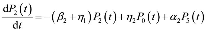
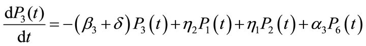

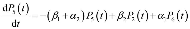
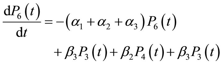 (1)
(1)
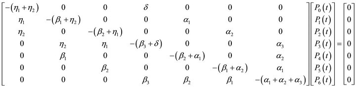
The above system of differential equations can be written in matrix form as
 (2)
(2)
where
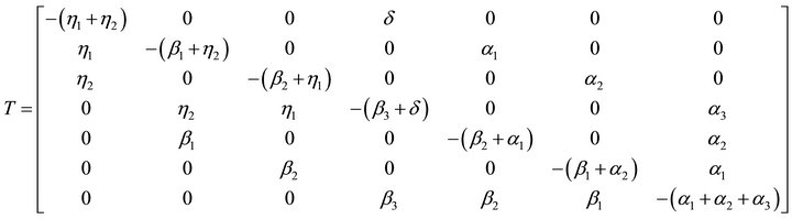
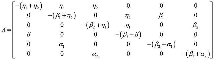
It is difficult to evaluate the transient solutions, hence we follow [4-6], the procedure to develop the explicit expression for MTSF is to delete the seventh row and column of matrix T and take the transpose to produce a new matrix, say A. The expected time to reach an absorbing state is obtained from
 (3)
(3)
where

4.2. System Availability Analysis
For the availability case of Figure 1 using the initial condition in Section 4.1 for this system,

The system of differential equations in (1) for the system above can be expressed in matrix form as:
Let  be the time to failure of the system. The steady-state availability is given by
 (4)
(4)
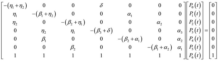
In steady state, the derivatives of state probabilities become zero, thus (2) becomes
 (5)
(5)
which in matrix form is
using the normalizing condition
 (6)
(6)
we substitute (6) in the last row of (5) following [4-6]. The resulting matrix is

We solve the system of linear equations in matrix above to obtain the state probabilities 
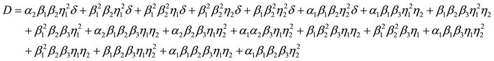
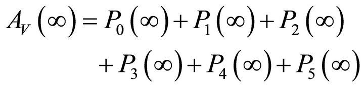
Expression for  thus is:
Computer programme (MATLAB) is used to develop the explicit expressions for the . The expression for the
  is lengthy to be shown here.
4.3. Busy Period Analysis
Using the same initial condition in Section 4.1 above as for the reliability case
and (5) and (6) the busy period is obtained as follows:
In the steady state, the derivatives of the state probabilities become zero and this will enable us to compute steady state busy period due to failure:
The system of differential equations in (1) for the system above can be expressed in matrix form as:
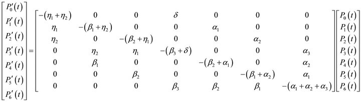
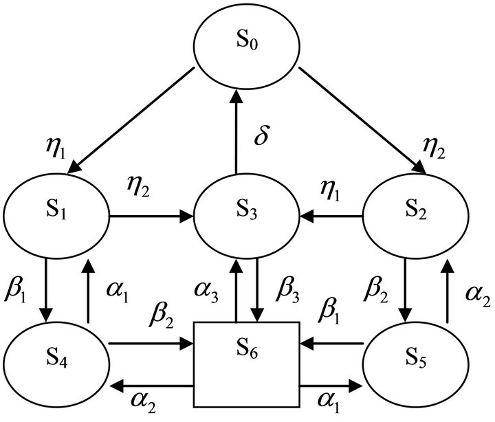
Figure 1. Schematic diagram of the system.
Let  be the probability that the repair man is busy either repairing the failed unit or exchanging the degraded units with new ones. The steady-state busy period is given by
 (7)
(7)
In steady state, the derivatives of state probabilities become zero, thus (2) becomes
 (8)
(8)
which in matrix form is

using the normalizing condition
 (9)
(9)
We substitute (6) in the last row of (5) (see [4-6]). The resulting matrix is
We solve the system of linear equations in matrix above to obtain the state probabilities 
Expression for  thus is:
 (10)
(10)
Computer programme (MATLAB) is used to develop the explicit expressions for the . The expression for the
  is lengthy to be shown here.
4.4. Profit Analysis
The system/units are subjected to corrective maintenance at failure as can be observed in states 4, 5 and 6. From Figure 1, the repairman is busy performing corrective maintenance action to the units at failure in states 4, 5 and 6. According to [4,5], the expected profit per unit time incurred to the system in the steady-state is given by:
Profit = total revenue generated – cost incurred for repairing the failed units.
 (11)
(11)
where : is the profit incurred to the system;
 : is the revenue per unit up time of the system;
 : is the accumulated cost per unit time which the system is under repair and unit exchange.
5. Results and Discussions
In this section, we numerically obtained the results for mean time to system failure, system availability, busy period and profit function for all the developed models. For the model analysis, the following set of parameters values are fixed throughout the simulations for consistency:
Case I: ,
,  ,
,  ,
,  ,
,  ,
,  ,
,  ,
,  ,
,  ,
,  ,
,  for simulations in Figures 2-16.
Case II: ,
,  ,
,  ,
,  ,
,  ,
,  ,
,  ,
,  ,
,  for simulations in Figures 17-21.
The impact of  on MTSF, steady-state availability, profit and busy period can be observed in Figures 3, 6, 14 and 19. From Figures 3, 6 and 14, it is evident that the MTSF, steady-state availability profit increases as
  increases while in Figure 19 as
  increases, the busy period of the repair man decreases. Similar results can be observed in Figures 2, 7, 13 and 17 on MTSF, steady-state availability, profit and busy period with respect to
 . From Figures 2, 7 and 13, MTSF, steady-
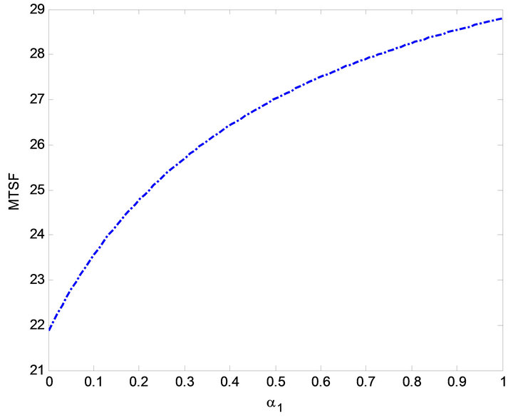
Figure 2. Effect of  on MTSF.
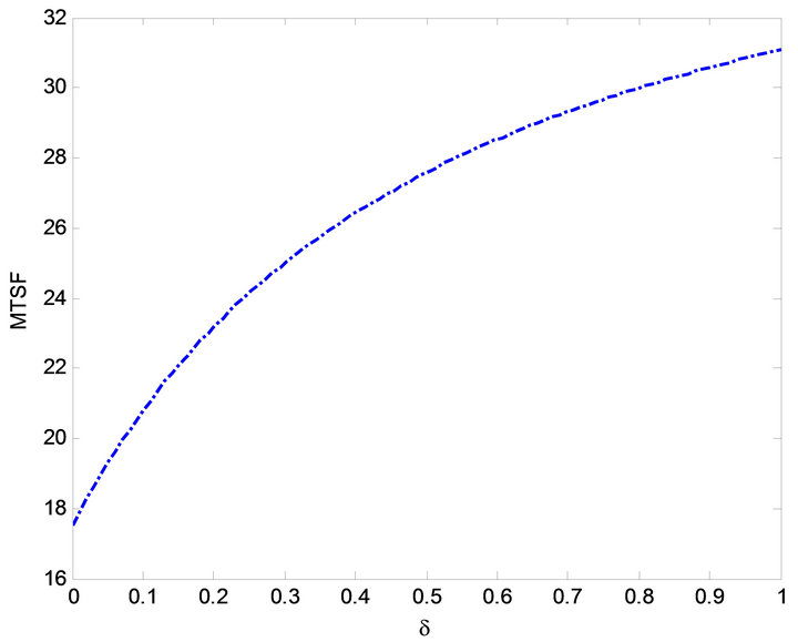
Figure 3. Effect of  on MTSF.
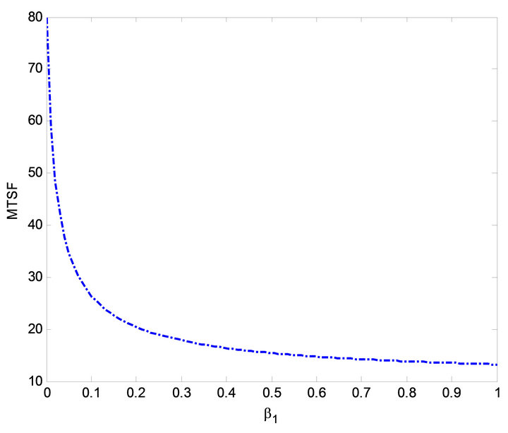
Figure 4. Effect of  on MTSF.
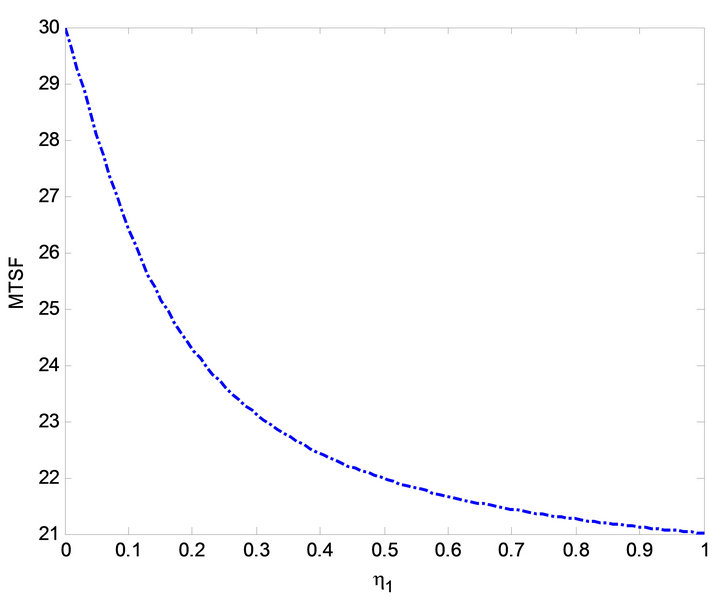
Figure 5. Effect of  on MTSF.
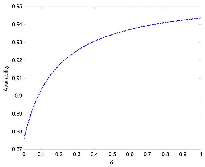
Figure 6. Effect of  on availability.
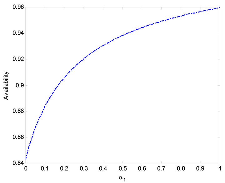
Figure 7. Effect of  on availability.
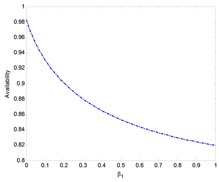
Figure 8. Effect of  on availability.
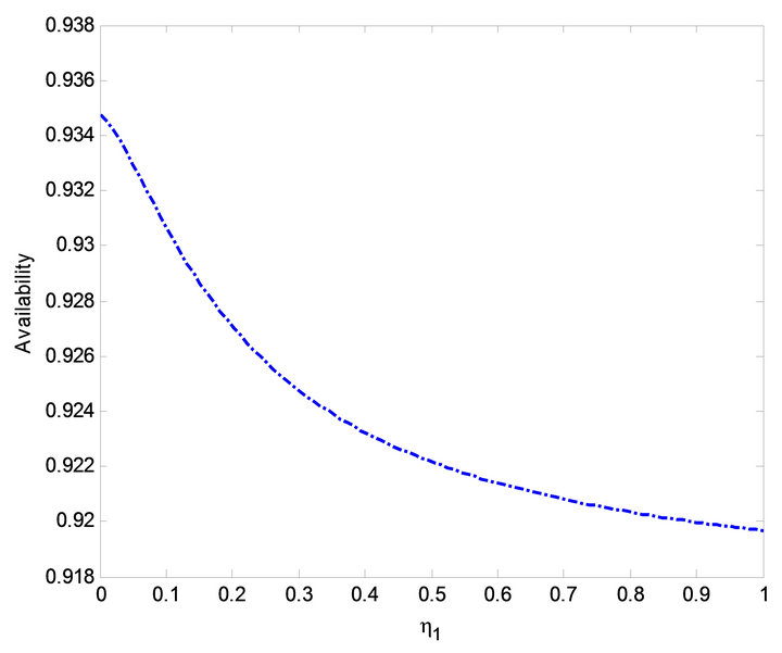
Figure 9. Effect of  on availability.

Figure 10. Effect of  on availability.
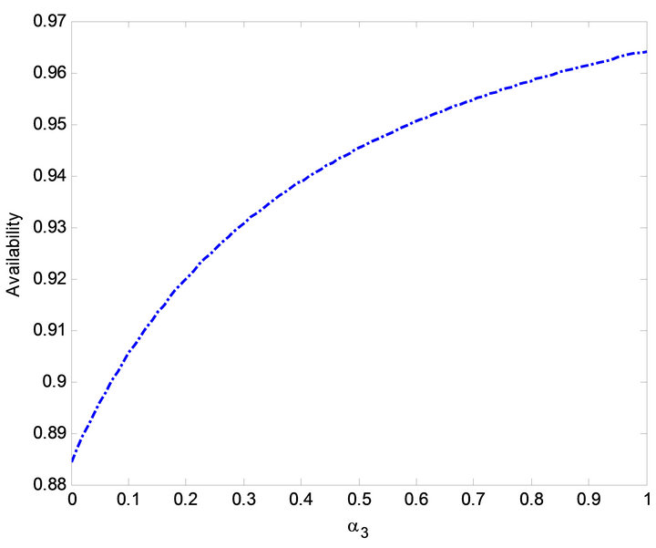
Figure 11. Effect of  on availability.
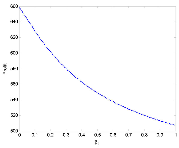
Figure 12. Effect of  on profit.
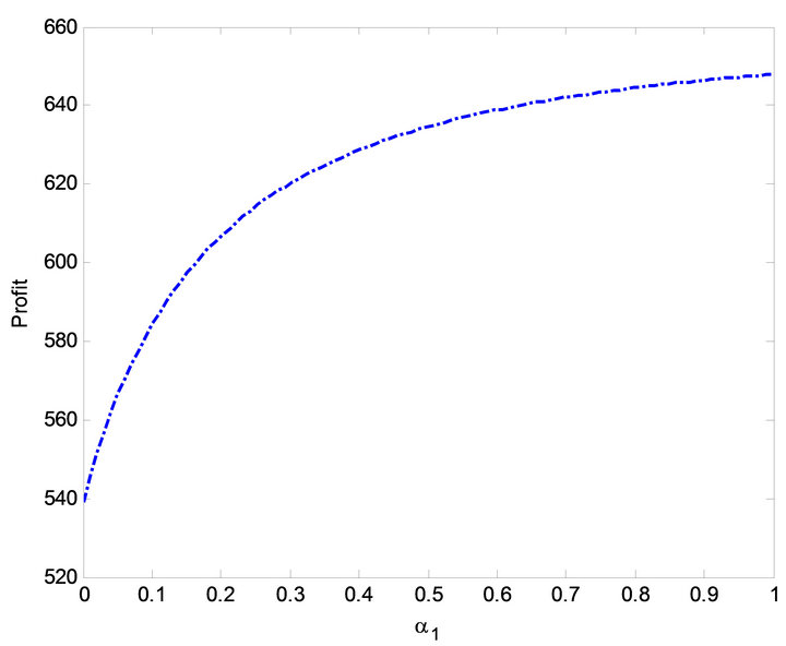
Figure 13. Effect of  on profit.
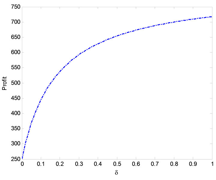
Figure 14. Effect of  on profit.
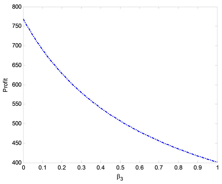
Figure 15. Effect of  on profit.
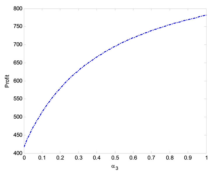
Figure 16. Effect of  on profit.
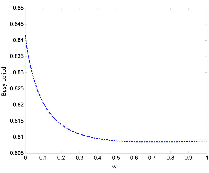
Figure 17. Effect of  on busy period.
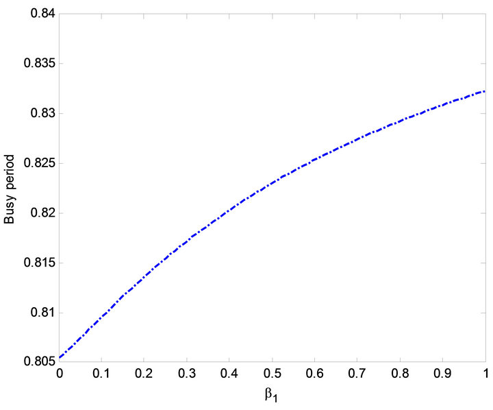
Figure 18. Effect of  on busy period.
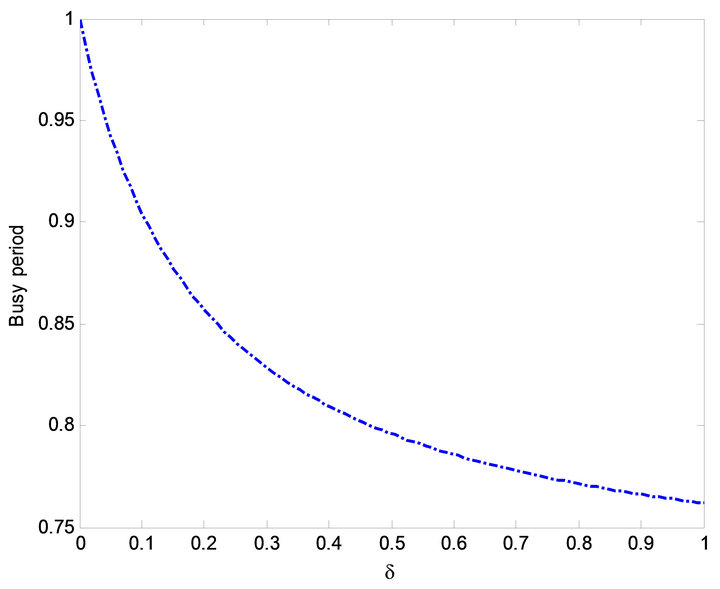
Figure 19. Effect of  on busy period.

Figure 20. Effect of  on busy period.
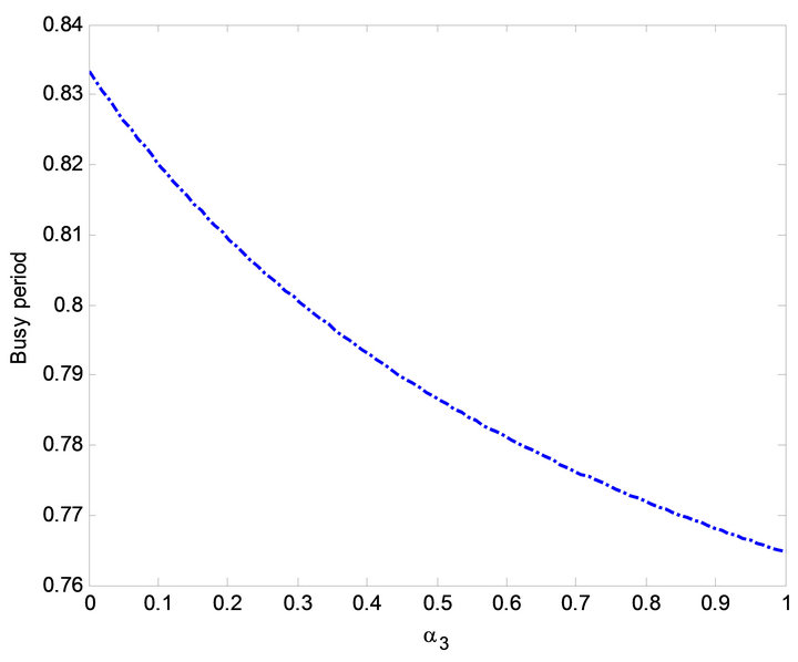
Figure 21. Effect of  on busy period.
state availability and profit increases as  increases while the busy period decreases with increase in
  from Figure 13. Results of MTSF, steady-state availability, profit and busy period with respect to
  are given in Figures 4, 8, 12 and 18. It is evident from Figures 4, 8 and 12 that as
  increases, the MTSF, steady-state availability and profit decreases while from Figure 18 the busy period increases with increase in
 . Furthermore, the impact of
  on MTSF and steady-state availability can be seen in Figures 5 and 9. In these figures, the MTSF and steady-state availability decrease as
  increases. Moreover, results of
  and
and  can be seen in Figures 10, 15, and 20 and Figures 11, 16 and 21 respectively. It is evident from Figures 10 and 15 that the steady-state availability and profit decreases as
  increases while in Figure 20, busy period increases with increase in
 . Simulation results of steady-state availability, profit and busy period can be observed in Figures 11, 16 and 21. In Figures 11 and 16, the steadystate availability and profit increases as
  increases while the busy period decreases with increase in
  from Figure 21.
6. Conclusion
In this paper, we constructed a linear consecutive 2-outof-3 repairable system operating in reduced capacity before failure. We have developed the explicit expressions for the MTSF, availability, busy period and profit function. We perform a parametric investigation of various system parameters on MTSF, system availability, busy period and profit function and captured their effect on MTSF, availability, busy period and profit function. These are the main contribution of the paper.
REFERENCES
- R. K. Bhardwaj and S. Chander, “Reliability and Cost Benefit Analysis of 2-out-of-3 Redundant System with General Distribution of Repair and Waiting Time,” DIAS-Technology Review—An International Journal for Business and IT, Vol. 4, No. 1, 2007, pp. 28-35.
- S. Chander and R. K. Bhardwai, “Reliability and Economic Analysis of 2-out-of-3 Redundant System with Priority to Repair,” African Journal of Mathematics and Computer Science Research, Vol. 2, No. 11, 2009, pp. 230- 236.
- R. K. Bhardwai and S. C. Malik, “MTSF and Cost Effectiveness of 2-out-of-3 Cold Standby System with Probability of Repair and Inspection,” International Journal of Engineering Science and Technology, Vol. 2, No. 1, 2010, pp. 5882-5889.
- K. Wang, C. Hsieh and C. Liou, “Cost Benefit Analysis of Series Systems with Cold Standby Components and a Repairable Service Station,” Journal of Quality Technology and Quantitative Management, Vol. 3, No. 1, 2006, pp. 77-92.
- K. M. El-Said, “Cost Analysis of a System with Preventive Maintenance by Using Kolmogorov’s Forward Equations Method,” American Journal of Applied Sciences, Vol. 5, No. 4, 2008, pp. 405-410. doi:10.3844/ajassp.2008.405.410
- M. Y. Haggag, “Cost Analysis of a System Involving Common Cause Failures and Preventive Maintenance,” Journal of Mathematics and Statistics, Vol. 5, No. 4, 2009, pp. 305-310. doi:10.3844/jmssp.2009.305.310
- K. H. Wang and C. C. Kuo, “Cost and Probabilistic Analysis of Series Systems with Mixed Standby Components,” Applied Mathematical Modelling, Vol. 24, No. 12, 2000, pp. 957-967. doi:10.1016/S0307-904X(00)00028-7
- K. C. Wang, Y. C. Liou and W. L. Pearn, “Cost Benefit Analysis of Series Systems with Warm Standby Components and General Repair Time,” Mathematical Methods of Operation Research, Vol. 61, No. 2, 2005, pp. 329- 343.
- M. A. Hajeeh, “Availability of a System with Different Repair Options,” International Journal of Mathematics in Operational Research, Vol. 4, No. 1, 2012, pp. 41-55. doi:10.1504/IJMOR.2012.044472
- H. S. Fathabadi and M. Khodaei, “Reliability Evaluation of Network Flows with Stochastic Capacity and Cost Constraint,” International Journal of Mathematics in Operational Research, Vol. 4, No. 4, 2012, pp. 439-452. doi:10.1504/IJMOR.2012.048904
NOTES
*Corresponding author.