Applied Mathematics
Vol. 4 No. 5 (2013) , Article ID: 31226 , 5 pages DOI:10.4236/am.2013.45105
The Stationary Distributions of a Class of Markov Chains
School of Mathematics and Statistics, University of Sheffield, Sheffield, UK
Email: c.cannings@shef.ac.uk
Copyright © 2013 Chris Cannings. This is an open access article distributed under the Creative Commons Attribution License, which permits unrestricted use, distribution, and reproduction in any medium, provided the original work is properly cited.
Received February 28, 2013; revised March 28, 2013; accepted April 5, 2013
Keywords: Parker’s Model; Markov Chains; Integer Sequences
ABSTRACT
The objective of this paper is to find the stationary distribution of a certain class of Markov chains arising in a biological population involved in a specific type of evolutionary conflict, known as Parker’s model. In a population of such players, the result of repeated, infrequent, attempted invasions using strategies from , is a Markov chain. The stationary distributions of this class of chains, for
  are derived in terms of previously known integer sequences. The asymptotic distribution (for
![]() ) is derived.
) is derived.
3. The Stationary Distribution
Now the dominant eigenvalue is m, and we derive a recurrence relation for the corresponding left eigenvector , the stationary distribution, where we set the right-most element equal to 1. It is straightforward to demonstrate that the final three elements of the eigenvector
  are
are ,
,  and 1.
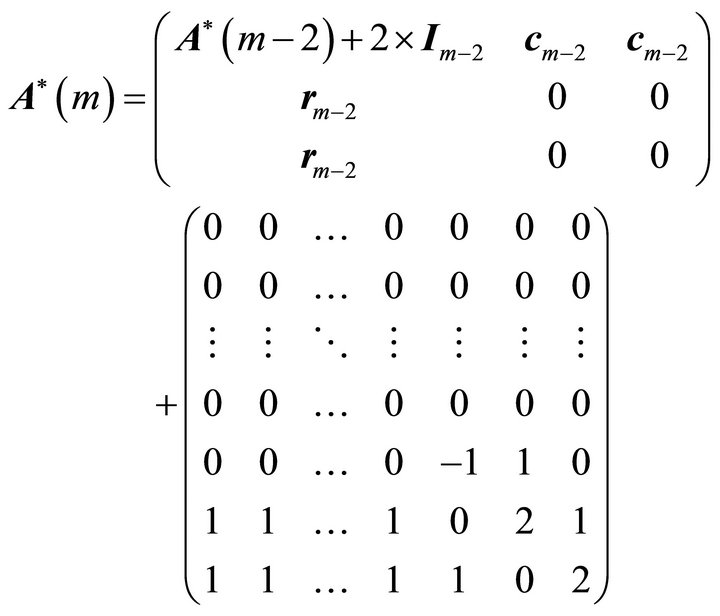
Observe that

where, throughout,  is the
  identity matrix,
  is a k element column vector and
 ![]() is a k element row vector.
is a k element row vector.
We then have
 .
.
Also
and so
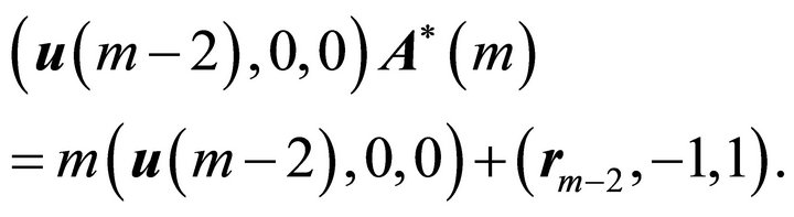
Now consider

We have
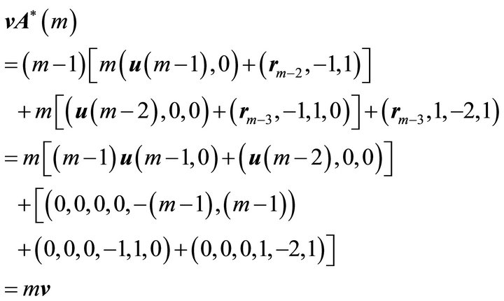
so ![]() is the required eigenvector.
is the required eigenvector.
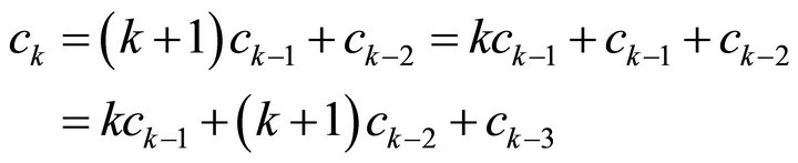
We now have a recurrence relation for the  which is
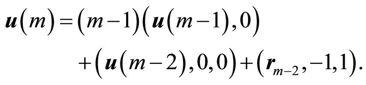
This is valid for  using
using  and
and
 .
.
Suppose we write  for the sum of the elements of
  so that
  is the stationary distribution of the Markov chain. We have immediately that
with ,
, . This is sequence A001040 [5] specified as
 , where our
  where the sequence is initiated with
  and
and .
.
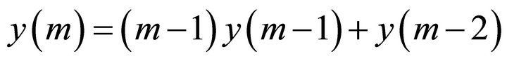
We can extract individual elements of the stationary distributions. Suppose that  is the i’th element of
 . Then we have that
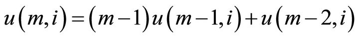
for ,
,  , with initial values
  and
and ,
,  and
and  and for
 , we have
  and
and . The sequence for
  is A058307, and
  is A058279 in [5].
Table 1 gives some values of .
.
4. The Asymptotic Eigenvector
Having derived recurrence relations for the elements of the eigenvectors we now consider the limit as![]() . We begin with a simple Lemma.
. We begin with a simple Lemma.
Lemma
Suppose we have a recurrence relation of the form  where the
  is not dependent on the
 , and
, and . Suppose we have two sequences,
  and
and  satisfying the recurrence relationship but initiated by different values i.e. by
  and
and  respectively. Then
  as
as  where
where ![]() is a constant, which depends on the initial values.
is a constant, which depends on the initial values.
Proof
Since

We have
Now the denominator increases at a rate greater than
 as one can see easily by considering the liniting case
 , so the above expression tends to zero as
  and so
  as
as .
.
Comment Much weaker conditions are necessary than those stated above for  as
as .
.
We can apply the lemma immediately to the elements of the stationary distribution, expressed in the integer form. The ratios for 0 and 1 elements for  are 1,
  , 1.307692, 1.308824, 1.308789, 1308789 illustrating the speed with which convergence takes place. We have no expression for the asymptotic value but for m = 200 the ratio is approximately 1.3087893731. The ratios for 1 and 2 elements for
  are 1, 0.5, 0.529412, 0.528090, 0.528131, 0.0.528130 and for m = 200 approximately 0.5281297672.
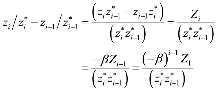
In the absence of a simple way of evaluating the limiting ratios discussed above analytically we adopt a different method to derive the asymptotic stationary distribution, again expressed in integers. Suppose this is given by , and define
 . We have that
 . Thus
 , and
, and
 .
.
In a similar way we can obtain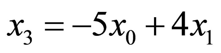 , and
, and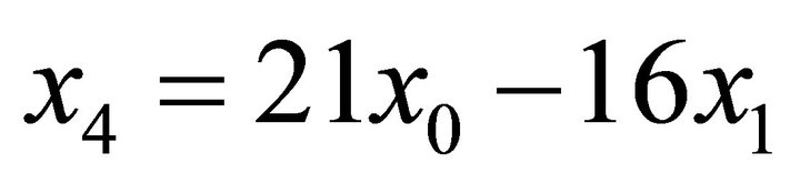 , and so on. It is clear that the signs alternate. For ease we introduce the following notation; we write
  when
when 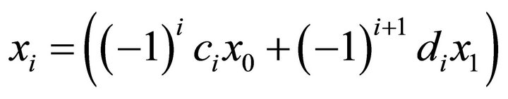 so that the sequences
  and
and ![]() for
for  consist of positive integers. Similarly we write
when  so the sequences
 and
and  consist of positive integers. Thus we have
 ,
,  ,
,  ,
,  ,
,  and so on, while
 ,
,  ,
,  and so on.
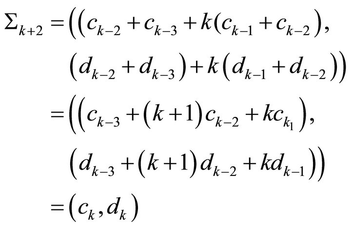
The theorem below gives recurrence relations for![]() ,
,  ,
,  and
and![]() , in terms of A058279 and A058307 [5].
, in terms of A058279 and A058307 [5].
Theorem
For  we have
  where
where
 with
with  ([5] A058279)
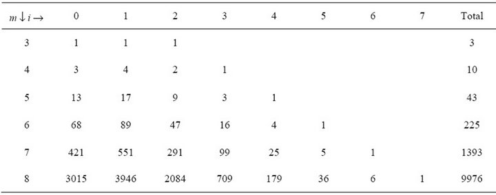
Table 1. Eigenvectors for m = 3(1)8.
and 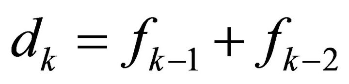 where
where 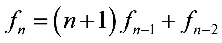 with
with  and
and  ([5] A058307). Further
  and
and .
.
Proof
We have that 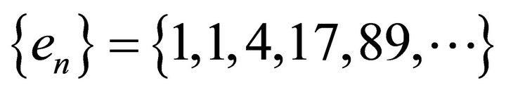 and
and 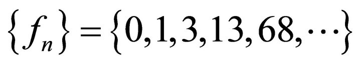 , and we have already shown that
 ,
,  ,
,  ,
,  ,
,  which satisfy the formula given in the statement of the theorem.
We prove that if the formula holds for  for
for  then it holds for
  for
for , and thence for
  for
for . Thence by induction.
Note first that
Suppose then that the formula for  holds for
 . Then since
  we have
  and substituting for the expressions given in the statement of the theorem we have
Now clearly we also have  so we have
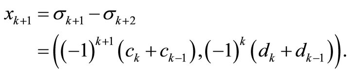
Table 2 gives the first 15 elements for the eigenvector for . Some idea of the speed of convergence can be gained by observing that these values agree with the elements of the eigenvector for
  except in the final 2 decimal places.
5. Conclusion
We have derived the stationary distribution of the frequencies of the available strategies in a population in which mutations occur infrequently, for Parke’s model when the reward is 2+ and for integer valued strategies. These relate to certain known integer sequences. This work provides a base for further investigations for other values of the reward, and more complex invasion processes.
6. Discussion
Parker’s model, which is also known as the Scotch Auction, is often used in the conflict theory literature as an example of a simple model in which there is no ESS (evolutionarily stable strategy). The implication of this is that there is no population assembly which is resistant to invasion. Of course if such a contests actually occurs it is important to ask what will happen in the population. This is the question which is addressed in [3], and which generates the class of matrices considered here. The stationary distribution then corresponds to the frequency with which one would observe a population to be playing a specific strategy, except if one happened on a population in transition.
The class of cases discusses above arises from Parker’s model when we consider a fixed reward value , and when the value of m, the range of possible strategies, is allowed to vary. It would be of interest to examine
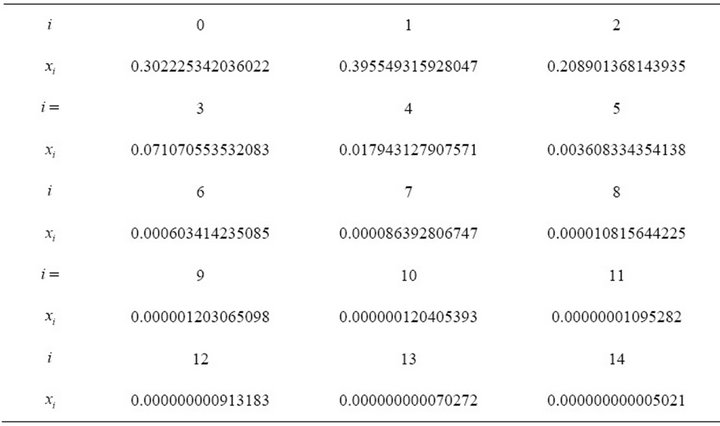
Table 2. First 15 eigenvector elements for m = 200.
other possible values of V as m varies. For example, for , the “Markov matrices” have 1’s for
  , 0’s for
  and diagonal elements to make the row sums m. It is hoped to treat these models in a subsequent paper.
We observe from the numerical values that the most frequent strategy value played is 1, that the distribution is uni-modal and that the strategies  are played over 90% of the time; asymptotically approximately 0.90667 which agrees to five decimal places to the value for
 , while the mean value is asymptotically approximately 1.1207 which agrees to five decimal places to the value for
 . These latter figures confirm the rapidity of the convergence.
REFERENCES
- M. Broom and C. Cannings, “Evolutionary Game Theory,” In: Encyclopedia of Life Sciences, John Wiley & Sons Ltd, Chichester, 2010. http://www.els.net
- G. A. Parker, “Sexual Selection and Sexual Conflict,” In: M. S. Blum and N. A. Blum, Eds., Sexual Selection and Reproductive Competition, Academic Press, New York, 1979, pp. 123-166.
- C. Cannings, “Populations Playing Parker’s Model,” In: Preparation.
- J. Norris, “Markov Chains,” Cambridge University Press, Cambridge, 1998.
- “The On-Line Encyclopedia of Integer Sequences.” http://oeis.org