Applied Mathematics
Vol. 3 No. 2 (2012) , Article ID: 17387 , 7 pages DOI:10.4236/am.2012.32021
Numerical Simulation of Nonlinear Surface Gravity Waves Transformation under Shallow-Water Conditions
Taganrog Technological Institute, Southern Federal University, Taganrog, Russia
Email: iftikhar_abbasov@mail.ru
Received November 23, 2011; revised January 9, 2012; accepted January 17, 2012
Keywords: Equations of Shallow-Water; Numerical Modelling; Nonlinear Surface Gravity Waves; Transformation of Surface Wave Profile
ABSTRACT
This work considers the problems of numerical simulation of non-linear surface gravity waves transformation under shallow bay conditions. The discrete model is built from non-linear shallow-water equations. Are resulted boundary and initial conditions. The method of splitting into physical processes receives system from three equations. Then we define the approximation order and investigate stability conditions of the discrete model. The sweep method was used to calculate the system of equations. This work presents surface gravity wave profiles for different propagation phases.
1. Introduction
The research of surface gravity waves under shallow water conditions has a long history. The interest to wave propagation effects on liquid surface can be explained by sufficient popularity and availability of this physical phenomenon. Non-linear surface gravity waves under shallow water conditions are described with shallow-water equations. They became the starting point of non-linear wave propagation effect study. In spite of a great number of studies, the liquid wave motion theory remains to be investigated. In this context the study of wave propagation effects on shallow water area surfaces taking account of their influence on coast formations and hydrotechnical constructions is of vital importance. Thus non-linear surface gravity wave simulation can play the important role when monitoring the ecological state of shallow bays.
Let us discuss the results of some studies, devoted to wave process numerical simulation within shallow water theory based on non-linear and non-linear-dispersion shallow water equations, pursued in the past decades.
The problems of monochromatic wave transformation above horizontal beach bottom were studied rather comprehensively in the papers by [1] and [2]. The first four harmonics influence on surface wave profile with its propagation on shallow water was studied in laboratory experiments and using numerical simulation. Evolutionary equation system was solved with Runge-Kutta method numerically. The model was verified and checked with the data of laboratory and real experiments.
Numerical simulation of non-steady periodic surface waves is described in the paper by [3]. The surface wave evolution problem is reduced to the solution of differential equation system. Ggravity wave dynamics is simulated numerically in amplitude variations and with different wavelengths. The gravity wave profiles are given at the initial instant and at the breaking moment.
Paper [4] considers numerical simulation and experimental observations of non-linear interaction, reflection and attenuation effects influencing the beach propagation of surface gravity waves. Non-linear interactions result in wave crest doubling. But for the waves with the less amplitude the wave crests do not double. The described effects are viewed within Boussinesq model.
Article [5] concerns non-linear long wave numerical simulation in the water bodies with a gentle bottom. Shallow water non-linear dispersion model is viewed considering the topography and fluid viscosity. They carry out a calculation comparison between free surface plane disturbance transformation and experimental data. This article presents numerical solution of the problem concerning conic-cylindrical island, sea ridge influence on the wave propagation. It considers the influence of slope bottom friction on plane solitary wave evolution as well.
Work [6] is concerned with the study of two-dimensional numerical influence model of flooded break wall on the wave propagation. It discusses the problems of wave simulation as before wave breaking so after it. The results of laboratory experiments are given to check the model. This work analyzes wave profile transformation. It also describes the dependence of wave steepness on its spectral structure.
Article [7] describes surface wave non-linear dispersion under shallow water conditions within Boussinesq model. The linear model was obtained as the first-order solution; at the second approach the model contains weak frequency and amplitude dispersion. The article presents experimental data on surface waves for a slope sand coast. Non-linear Boussinesq theory fully describes irrotational wave motion within breaker zone.
Work [8] offers a stochastic model of surface wave propagation under shallow water conditions with regard to the bottom topography. In the beginning it describes determined spectral model based on wave spectrum decomposition. It compares the developed model with the known analytic expressions for deep-water and shallowwater modes. There are also laboratory observations on non-linear wave propagation given in this work.
Paper [9] discusses the problem of single surge wave stability on Korteweg-de Vries equation. They use Whitham modulation theory for asymptotic description of surface swelling. They obtain an expression to describe the dependence of solitary wave form and amplitude on depth function.
In article [10] algorithm for an asymptotic model of wave propagation in shallow-water is proposed and analyzed. The algorithm is based on the Hamiltonian structure of the equation, and corresponds to a completely integrable particle lattice. Particle trajectories on the (x,t) plane are presented.
Analyzing the works described above, one could note the iterative solution methods of discrete equations are used in major cases. In our case we shall use precise solution methods of discrete shallow-water equations under hydrophysical conditions of the Azov Sea.
2. System of Shallow Water Equation. Initial and Boundary Condition
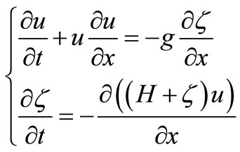
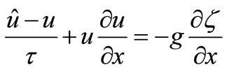
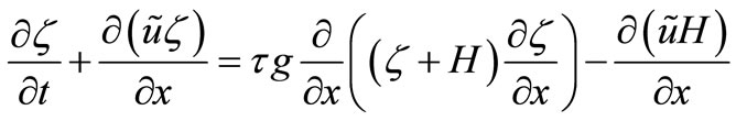
The surface gravity waves under shallow water conditions are described by the shallow-water equation. The system of shallow water equations contains a continuity equation and dynamic equation on the conservation of momentum [11,12]:
 (1)
(1)
where u—medium particle velocity, ζ—surface swell function, H—fluid depth. Shallow water equations ignore the dispersion phenomenon as it is of minor importance in shallow water.
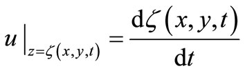
The kinematic boundary condition is taken as a boundary condition on free liquid surface, i.e. surface swelling velocity is the same as medium particle vertical velocity:
 (2)
(2)
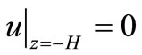
To follow the dynamic condition, the free liquid surface pressure is considered the same as the atmospheric pressure. As a bottom condition, vertical intensity of liquid particle velocity is assumed to be equal to zero:
 (3)
(3)
At the time zero the initial condition is assumed to be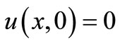 , at any other time the change in the surface form is given according to the harmonic law
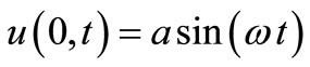 , where a, ω—surface wave amplitude and circular surface wave frequency.
3. Discrete Model Construction
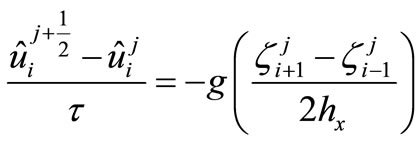
For the first equation of the system (1) we write the discrete analogue derivative in the time coordinate:
 (4)
(4)
We shall apply the method of splitting into physical processes for the Equation (4)
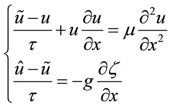 (5)
(5)
where![]() —a velocity component on the current time layer;
—a velocity component on the current time layer; —a velocity component on the auxiliary time layer;
 —a velocity component on the next time layer, τ—a time step, μ—a lattice velocity parameter.
Let us multiply the second system Equation (5) by
(H + ζ) and take the derivative in x—time coordinate of both members:
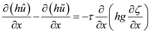 (6)
(6)
In view of the second system Equation (1), the Equation (6) may be written as:
 (7)
(7)
The expression is a constraint equation of level swelling function ζ and velocity component  on the auxiliary time layer.
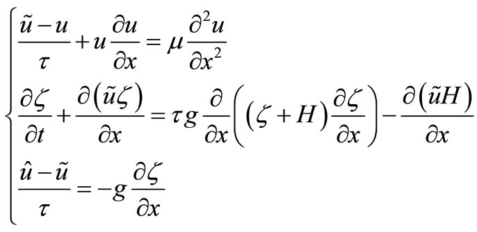
Thus the system of Equations (1) changes to:
 (8)
(8)
The operational algorithm of the system of Equations (8) is the following:
• from the first equation one finds the components on the auxiliary time layer— , through velocity components on the current time layer—
![]() ;
;
• then, from the second equation one finds level swelling function—ζ;
• finally, from the third equation one finds velocity components on the next time layer— .
.
Extra viscosity factor μ (0 < μ < 1) has been introduced into the system of shallow water Equations (8) when splitting into physical processes. Shallow water equations are hyperbolic systems of equations. Non-linear hyperbolic equations, compared to linear equations, possess a number of vital differences. These differences should be not overlooked in their numerical integration. Even if the initial conditions are as smooth as desired, the solution of non-linear equations can contain discontinuities.
In order to avoid this difficulty in practical solving of the problems of nonlinear mechanics, a small additional perturbation in the form of artificial viscosity is introduced into the differential system (similar to Von Neumann-Richtmyer Method) [13]. This viscosity eliminates discontinuities and leads to adequate results.
Difference scheme is used to solve numerically differential equations. The difference scheme is based on the integro-interpolation method on a uniform grid according to the implicit scheme [14,15]. The implicit scheme has been chosen for its greater stability factor выбрана.
The discrete analogues of the system of Equations (1) will be the following equations:
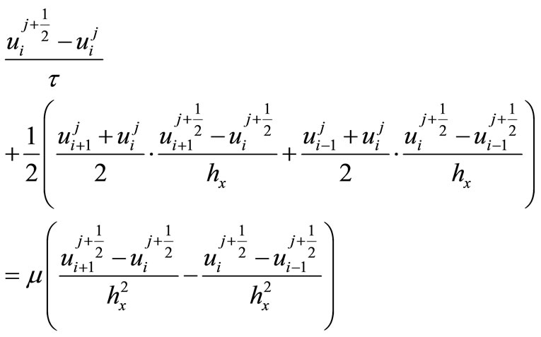 (9)
(9)
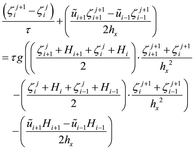 (10)
(10)
 (11)
(11)
For defining the approximation order is used the decomposition in Taylor rows of functions velocity components and level swelling concerning knot (j) and (j + 1). For difference operators we will receive:
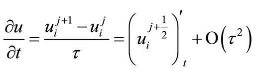 , (12)

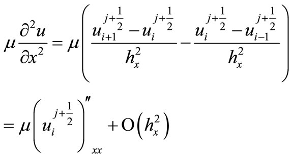
As a result the continual problem is equivalent to the discrete problem with the following approximation order: , where hx—step in the spatial coordinate.
The approximation condition is not sufficient for reception of the precise solution at step reduction. For such schemes maintenance of stability condition is necessary still. It is possible to present these schemes as some linear operator. It will transform function values at the moment t to function values at the moment of t + h. The stability condition demands, those values of this operator did not exceed in module 1 + ch, where c-constant. At default of the given condition an error of the scheme quickly increase and the small step, the less precise result. If approximation and stability conditions are satisfied the result difference schemes converges to the solving the differential equation. According to the Courant-FriedrichsLevy condition grid steps are limited by the following expression: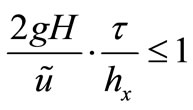 .
.
For the calculating the discrete equations one of economic direct methods—a sweep method is used. The sweep method represents a variant of Gauss method. It is applied to special systems the linear algebraic equations with tape structure of matrix.
The program has been developed for calculation of functions velocity components and level swelling. The program has been made and realized in language C++ in operational system Windows Vista.
4. Simulation of Non-Linear Surface Gravity Wave Propagation under Bay Conditions
Let us consider simulation features of surface gravity wave propagation under shallow-water conditions. Some hydrophysical data of shallow water area are required for simulation. We shall use the conditions of the Gulf of Taganrog of the Azov Sea (as it is geographically available) as a shallow water area. Though, hydrophysical conditions of other shallow water areas can be used.
The Azov Sea and its subsurface relief were formed at drowning of the Azov-Kuban basin. The Azov Sea is an interior sea, its shape is comparatively simple, its coasts are relatively regular and the bottom configuration is rather simple. The Azov Sea is surrounded by escarpment and spit forms. The smooth coast grades to plane and flat bottom. The inmost depths are in the central part of the sea. The inmost depth of the Azov Sea is 14 m, and the mean depth is about 8 m [16].
There are ten bays in the Azov Sea; three of them are of the closed type: the Gulf of Taganrog, the Sivash and the Gulf of Taman. In the North-East the strongly desalted Gulf of Taganrog is connected with the sea by the wide strait between the Belosarayskaya and Dolgaya Spit. The least gulf’s width (about 26 km) is stated between the Petrushina Spit and the Tchumburskaya Spit. The gulf’s bottom is intensely receding from the delta of the Don River to the sea; the average underwater gradient is 0.06%. To the West of Taganrog the gulf depth reaches 5 m, and it is less than 1 m near the Don’s delta [17].
In the Azov Sea wave motions are firstly shown as wind waves. They quickly develop, and after 2 hours the wind appears, reach the steady state. On the high seas, as a rule, short and very steep waves appear. Through the cold part of the year the reigning North-East and East winds cause very rough sea, with the wave height growing to 2.1 m, even 3.0 m. More often wave length reaches 10 - 12 m and wave height is from 0.5 m up to 1 m.
Figure 1 shows the results of numerical calculations
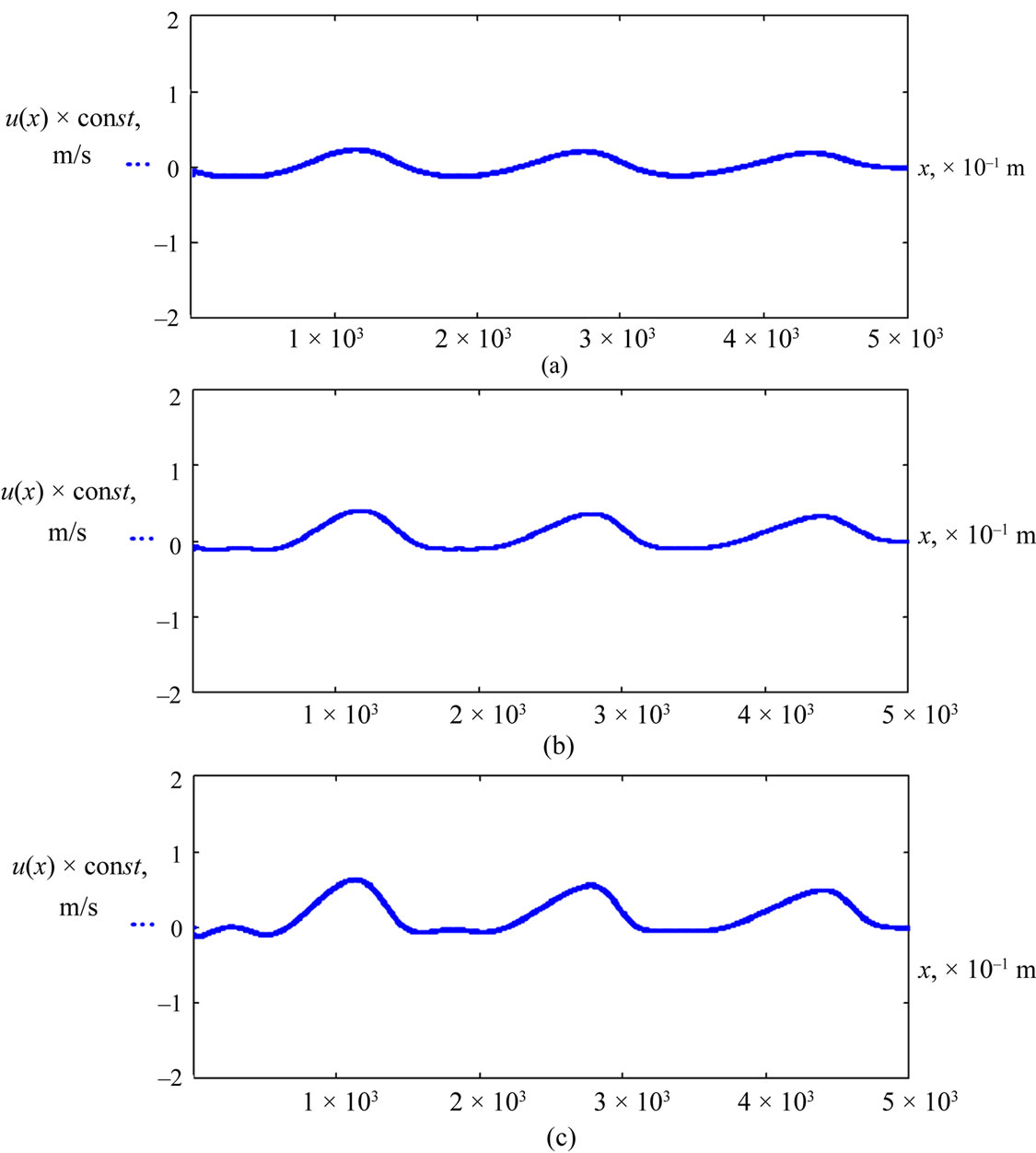
Figure 1. The profile dependence of surface gravity wave on the initial steepness: Frequency f = 0.045 Hz; wave length l = 155.6 m; depth H = 5 m; velocity c = 7 m/s; kH = 0.2; (а) 2a/l = 0.0024; ε = 0.04; (b) 2a/l = 0.0039; ε = 0.06; (c) 2a/l = 0.006; ε = 0.09.
for particle velocity of a surface gravity wave for different values of initial wave steepness ratio. Surface wave parameter values are adapted to the bathymetrical conditions of the Gulf of Taganrog. For calculations the depth values within 0.5 ≤ H ≤ 5 m are used. And the depth value is kept constant for specific conditions. In our case the surface gravity waves are free, i.e. they are ripples, so we neglect the wind effect.
For our conditions surface gravity waves are considered to be shallow under the following condition [11]: , where
![]() —surface gravity wave length. The lengths of surface gravity waves should be fully 2 times longer than the shallow water depth. Then for the conditions of the Gulf of Taganrog the surface gravity waves with the lengths more than 30 m can be considered as shallow.
—surface gravity wave length. The lengths of surface gravity waves should be fully 2 times longer than the shallow water depth. Then for the conditions of the Gulf of Taganrog the surface gravity waves with the lengths more than 30 m can be considered as shallow.
For the calculations we used the grid with number of points n = 5000, the node capacity for the wave length is 1556, width value in space hx = 0.1 m, shallow water parameter H/λ = 0.032, non-linear parameter ε = a/H. The profile of sine surface wave in Figure 1 does not suffer special changes on its propagation way. With the growth of surface wave steepness the original sine profile is changing, primarily valleys become sloping (Figure 1(b)), further on an intermediate crest appears in the valley. On its propagation way the intermediate crest is flattening and, the leading edge of the leading wave crest is steeping (Figure 1(c)).
With the less steepness the leading edge steeping is slow, i.e. it requires to accumulate non-linear effects at long distances. The increase of wave steepness value results in non-linearity increase and the surface wave comes to the leading edge steeping faster. The steeping of the surface wave leading edge is connected with the influence of non-linear term of shallow-water equations. Approaching the land the wave crest moves faster than a valley for its bottom friction. At the moment when “the crest is catching the trough up” the leading edge becomes vertical, and the wave breaks.
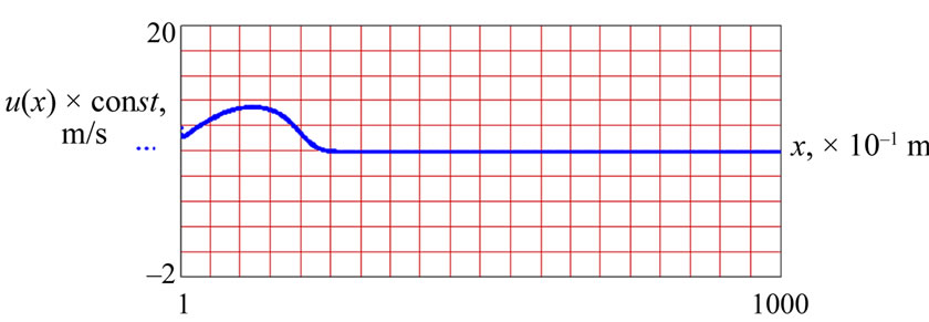
For more detailed monitoring of the leading edge steeping, Figure 2 shows the surface wave distortion stage by stage with the following parameters: frequency f = 0.045 Hz, length l = 49.2 m, depth H = 0.5 m. The depicted functional connections correspond to different time layers: t = 99; 199; 299; 399. The size of grid is n = 1000; the node capacity for the wave length is 492, width value in space hx = 0.1 m.
At the beginning of its propagation way t = 99 the surface wave crest is still sine, further on the valley starts falling behind and moves to the next crest t = 299. It results in steeping of the crest leading edges t = 399 (Figure 2(d)). When the leading edge is vertical, the wave starts breaking. The surface wave distortion is caused by the depth effect.
 (a)
(a)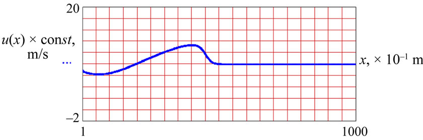 (b)
(b)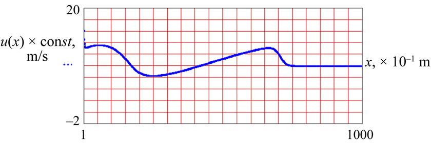 (c)
(c)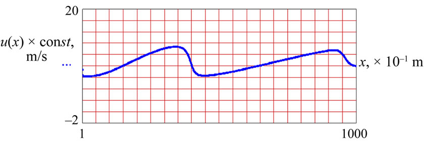 (d)
(d)
Figure 2. Gradual distortion of surface gravity wave profile: f = 0.45 Hz; l = 49.2 m; H = 0.5 m; c = 2.2 m/s; kH = 0.06; 2a/l = 0.0073; ε = 0.4; (а) time layer t = 99; (b) t = 199; (c) t = 299; (d) t = 399.
5. Analysis and the Result Comparison
To check the developed model let us compare our results with the results of laboratory and real experiments. Work [18] presents the results of laboratory experiment on the surface wave propagation above the step horizontal bottom with planes of different gradients. Article [6] shows numerical and experimental research on flooded breakwall influence on the surface wave propagation. Twodimensional finite-difference numerical model was made on the basis of Navier-Stokes equation.
To compare the results we shall use experimental and numerical profiles of surface waves given in the work by [6] (the length of laboratory tank is 30 m, width is 0.7 m, depth is 0.95 m, wave periods are T = 0.8; 1.2; 1.68 s).
Figure 3 shows the results of numerical simulation and experimental profiles of a surface wave on different propagation stages [6]. On their comparison with the developed model (Figures 1 and 2) one can note the following:

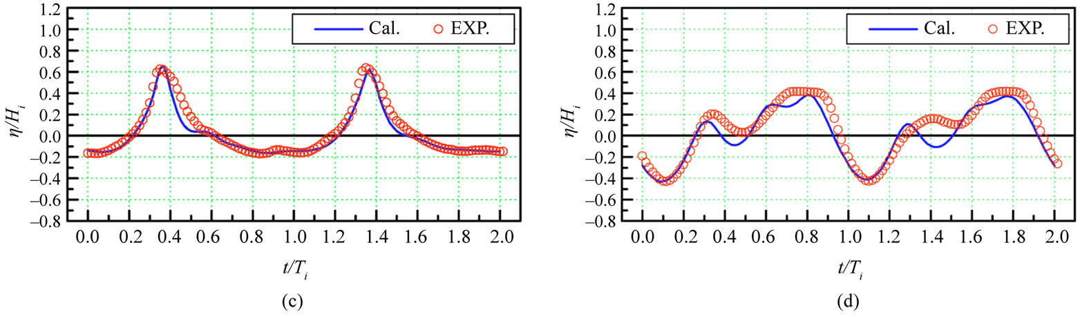
Figure 3. Estimated and experimental profiles of surface wave [6] (the coast is on the left): (2a/λ = 0.03, h/λ = 0.2; η(x)—surface swell function)); (a) at the beginning of the breakwall (x/λ = 0.1); (b) above the breakwall (x/λ = 0.3); (c) above the breakwall (x/λ = 0.4); (d) behind the breakwall (x/λ = 0.7).
• at the beginning of the breakwall surface wave experimental profiles start distorting as the depth decreases, the leading edge of the crest l starts steeping, valleys flatten (Figures 3(a) and (b));
• with further wave propagation above the breakwall the crests sharpen, the intermediate crest appears in a valley;
• in Figure 2(d) the surface wave (for depth influence) with further propagation transforms from sine into non-linear one with steep leading edge, as it was at the initial stage of experimental way in Figure 3(a);
• the growth of initial steepness for our model results in intermediate crest appearing in a valley Figure 1(c), it is analogue to the experimental profile, Figure 3(c);
• the depth increases behind the breakwall and the wave crests break up because of dispersion. This stage of wave profile transformation cannot be described by shallow-water equations. It should be also noted that primary processes of crest sharpening and its further leading edge steeping were described with the approximate analytics in the works by [19,20].
Finally, based on the comparison, one can note that the results of the numerical simulation of non-linear surface gravity waves on shallow-water equations agree reasonably well with experimental measurements.
REFERENCES
- G. Chapalain, R. Cointe and A. Temperville, “Observed and Modeled Resonantly Interacting Progressive WaterWaves,” Coastal Engineering Journal, Vol. 16, No. 3, 1992, pp. 267-300. doi:10.1016/0378-3839(92)90045-V
- Y. Eldeberky and P.A. Madsen, “Determenistic and Stochastic Evolution Equations for Fully Dispersive and Weakly Nonlinear Waves,” Coastal Engineering Journal, Vol. 38, No. 1, 1999, pp. 1-24. doi:10.1016/S0378-3839(99)00021-6
- V. R. Kogan and V. V. Kuznetsov, “Application of the Theory of Analytical Functions in Numerical Simulation of Unsteady Surface Waves,” Zhurnal Vychislitel’Noi Matematiki i Matematicheskoi Fiziki, Vol. 36. No. 10, 1995, pp. 1448-1456.
- S. Elgar, C. Norheim, T. Herbers, “Nonlinear Evolution of Surface Wave Spectra on a Beach,” Journal of Physical Oceanography, Vol. 28. No. 7, 1998, pp. 1534-1551. doi:10.1175/1520-0485(1998)028<1534:NEOSWS>2.0.CO;2
- А. А. Litvinenko and G. А. Habahpashev, “Numerical Simulation of Nonlinear Rather Long Two-Dimensional Waves in Basins with Gentle Bottom,” Vytchislitelnye Technologii, Vol. 4, No. 3, 1999, pp. 95-105.
- K. Kawasaki, “Numerical Simulation of Breaking and Post-Breaking Wave Deformation Process around a Submerged Breakwater,” Coastal Engineering Journal, Vol. 41. No. 3-4, 1999, pp. 201-223. doi:10.1142/S0578563499000139
- T. H. Herbers, S. Elgar, N. A. Sarap and R. T. Guza, “Nonlinear Dispersion of Surface Gravity Waves in Shallow Water,” Journal of Physical Oceanography, Vol. 32. No. 4, 2002, pp. 182-1193. doi:10.1175/1520-0485(2002)032<1181:NDOSGW>2.0.CO;2
- T. T. Janssen, T. H. Herbers 2002 and J. A. Battjes, “Generalized Evolution Equations for Nonlinear Surface Gravity Waves over Two-Dimensional Topography,” Journal of Fluid Mechanics, Vol. 552, 2006, pp. 393-418. doi:10.1017/S0022112006008743
- G. A. El, R. H. Grimshaw and A. M. Kamchatnov, “Evolution of Solitary Waves and Undular Bores in ShallowWater Ows over a Gradual Slope with Bottom Friction,” Journal of Fluid Mechanics, Vol. 585, 2007, pp. 213-244. doi:10.1017/S0022112007006817
- R. Camassa, J. Huang and L. Lee, “On a Completely Integrable Numerical Scheme for a Nonlinear ShallowWater Wave Equation,” Journal of Nonlinear Mathematical Physics, Vol. 12. No. 1, 2005, pp. 146-162. doi:10.2991/jnmp.2005.12.s1.13
- H. Lamb, “Hydrodynamics,” Dover Publications, Mineola, 1930, p. 524.
- G. B. Whitham, “Linear and Nonlinear Waves,” Wiley, New York, 1974, p. 622.
- R. Richtmyer and K. Morton, “Difference Methods for Initial-Value Problems,” 2nd Edition, Wiley, New York, 1967, p. 309.
- M. Holt, “Numerical Methods in Fluid Dynamics,” SpringerVerlag, New York, 1977, p. 305.
- А. А. Samarskyi, “Introduction to Numerical Methods,” Nauka, Glavnaja Redaktsija Fiziko-Matematicheskoi Literatury, Moscow, 1987, p. 288.
- “Hydrometeorology and Hydrochemistry of the Seas in the USSR,” Gidrometeoizdat, Vol. 5, The Azov Sea, Saint-Petersburg, 1991, pp. 75-88.
- V. А. Mamykina and Yu. P. Khrustalev, “Coastal Zone of the Azov Sea,” Izdatelstvo Rostov State University, Rostov-on-Don., 1980, p. 176.
- Y. Goda and K. Morinobu, “Breaking Wave Heights on Horizontal Bed Affected by Approach Slope,” Coastal Engineering Journal, Vol. 40, No. 4, 1998, pp. 307-326. doi:10.1142/S0578563498000182
- I. B. Abbasov, “Study and Simulation of Nonlinear Surface Gravity Waves under Shallow-Water Conditions,” Izvestiya RAN, Atmospheric and Oceanic Physics, Vol. 39, No. 4, 2003, pp. 506-511.
- I. B. Abbasov, “Transformation of Nonlinear Surface Gravity Waves under Shallow-Water Conditions,” Applied Mathematics, Vol. 1, No. 4, 2010, pp. 260-264. doi:10.4236/am.2010.14032