Journal of Environmental Protection
Vol.08 No.11(2017), Article ID:79733,16 pages
10.4236/jep.2017.811080
Measurements and Visualization of the Fluid Field of the Plume from an Animal Housing Ventilation Fan
Manqing Ying1, Lingjuan Wang-Li1*, Larry F. Stikeleather1, Jack Edwards2
1Department of Biological and Agricultural Engineering, North Carolina State University, Raleigh, USA
2Department of Mechanical and Aerospace Engineering, North Carolina State University, Raleigh, USA

Copyright © 2017 by authors and Scientific Research Publishing Inc.
This work is licensed under the Creative Commons Attribution International License (CC BY 4.0).
http://creativecommons.org/licenses/by/4.0/


Received: August 21, 2017; Accepted: October 17, 2017; Published: October 20, 2017
ABSTRACT
Various dispersion models have been developed to simulate the fate and transport of air emissions from animal housing systems to meet the increasing need for knowledge in this area. However, the accuracy of the models may be challenged due to the unknown plume rise and plume shape. This paper reports a combination of theoretical and field study of the plum rise and shape of air flow from a ventilation fan commonly used in mechanically ventilated animal houses. The theoretical modeling of the plume shape was conducted using a commercial Computational Fluid Dynamics (CFD) package named FloEFD; the field measurements of the plume field was conducted using five 3D ultrasonic anemometers to simultaneously measure the air flow in the plume at various locations (four heights and five downwind distances). The TECPLOT package was used to visualize the plume flow field based upon anemometer measurements. While the plume shapes were found to be left-shifted by the CFD model and TECPLOT visualization, the magnitudes of the 3D wind velocities from field measurement were found to be significantly larger than those from CFD model. The plume field measurements indicated that the plume of a 0.6 m (24-inch) ventilation fan had a depth about 9 m, a width about ±6 m, and a rise (lifting) beyond the highest measurement point, 4.88 m (16 ft).
Keywords:
Computational Fluid Dynamics (CFD), Plume Fluid Field Measurement, Plume Rise, Animal Housing

1. Introduction
Animal products are more and more in need to feed the rapidly growing population. It has been reported [1] that there were 450,000 animal feeding operations (AFOs) in the United States. Along with the significant economic and social benefits produced by the AFO industry, however, serious environmental concerns have been raised due to massive production of animal waste and air emissions from the operations. In assessment of impact of AFO air emissions on local and regional air quality, knowledge of the fate and transport of those emissions is required, and yet has not been well studied and understood.
While estimations of air emissions from AFO facilities have been studies intensively [2] [3] [4] , investigation of the fate and transport of the emissions is a relatively newer research topic in recent years [5] [6] [7] [8] . In the literature, estimations of downwind pollutant concentrations in responses to AFO emissions have been commonly conducted through Gaussian dispersion modeling approach [8] [9] [10] . The Gaussian dispersion model was originally developed based upon observations of industrial “stack” emissions with vertical momentum and thermal buoyancy [11] . The accuracy of the Gaussian dispersion model may be challenged when it is applied for assessing dispersion of air emissions from animal housing system where there is lack of vertical momentum and sufficient “stack” height. This challenge mainly comes from unknown of plume rise and plume shape of the horizontal emissions from the housing ventilation fans.
The rise of the centerline of a dispersing plume is called the plume rise. Currently, the Briggs’ formula and the Holland’s formula [11] are most commonly used models to estimate the plume rises. Despite the fact that the estimation of these two plume rise models do not agree with each other, both the Briggs’ formula [5] and the Holland’s formula compute the plume rise by two parts: the rise caused by thermal lifting and the rise caused by vertical momentum.
Applying both Briggs and Holland formulas into the case of animal housing systems, a small plume rise would be expected due to the lack of vertical momentum and thermal buoyancy under warm weather condition. However, field observation showed that the plume rise of exhaust air from animal buildings could actually reach as high as 10 m (Figure 1). Moreover, unlike the plume rise

Figure 1. Plume of air emissions (mixture of PM + gas + moisture) from two tunnel ventilated poultry houses (Note: the background trees were over 14 m high) (image by Wang-Li).
models for industrial stacks used in the existing formulas, for AFO housing system, the emission “stacks” are much lower with horizontal initial air flow instead of vertical flow as compared to the industrial stacks. Thus, the accuracy of the existing formulas is challenged when applying to the case in animal housing system.
In an effort to assess an emission plume, Holmes et al. [12] reported that the flow patterns of gas and PM emissions agreed well in open environments unless there was severe turbulence or the emission sources were too complicated. Understanding of fluid filed of the exhaust plume from animal housing ventilation fans may lead to quantification of rises of the emission plumes. In theory, fluid dynamic equations, which are mostly in the forms of partial differential equations, may be used to express the fundamental principles of any fluid field and to predict fluid field behavior under any given boundary conditions [13] . To find a numerical description of the fluid field that meets the fundamental principles and the given boundary conditions, as much as millions of iterations could happen. To facilitate such high computational demand, the computational fluid dynamics (CFD) has been commonly used in fluid field calculation and modeling. In application of the CFD modeling, fluid field measurements are usually required to validate and calibrate the model outputs. While there are many publications about both CFD modeling and field measurements of industrial fan flows [14] [15] [16] , there is seldom comparison between them, especially for closer downwind fluid field studies. This is probably because, as Quinn et al. [17] concluded, the performance of the modeling systems depends highly on the fluctuation of the wind conditions.
In addition to CFD method for fluid field modeling, TECPLOT [18] is another fluid dynamic package to visualize and model the fluid field behavior when the fluid field measurements are available. It has been applied in visualization of various research fields such as heat transfer process [19] , flow field measurement [20] and even chemical reactions [21] .
This study compared the flow filed measurements with the CFD model outputs of the fluid field of the exhaust plume from a ventilation fan commonly used in AFO housing systems. The specific objectives of the research was to 1) measure the fluid field of the exhaust plume from an animal housing ventilation fan; 2) visualize and quantify the shape and rise of the plume through CFD modeling and TECPLOT visualization.
2. Methodology
In this study, two approaches were taken to model and visualize rise of the plume emitted from a ventilation fan testing setup. The first approach measured fluid field of the ventilation plume under the controlled setting. The fluid field measurements were then applied to TECPLOT to visualize the exhaust plume shapes defined by plume height, depth and width. In the second approach, a commercially available CFD package (FloEFD 11 for Creo, Mentor Graphics) was used to simulate the fluid field of the plume emitted from the ventilation fan testing setup. Through the plotting of the model resulted by CFD approach, plume rise and shape was then observed and quantified.
2.1. Ventilation Plume Testing Setup: The Mini-Tunnel
To be consistent with field observation, a wooden mini-tunnel with an axial ventilation fan was constructed to simulate ventilation flow that would be typically observed in a poultry housing system. This testing mini-tunnel has a dimension in 1.22 m × 0.91 m × 2.44 m (4 ft × 3 ft × 8 ft) with an axial ventilation fan (0.6 m, 24” in diameter, AT24ZCP, Aerotech) installed on the one end. To ensure similar air flow pattern in the testing tunnel as it is in a typical poultry house, a collimating screen was installed at the entrance end of the tunnel. This collimating screen not only stabilized the airflow in the tunnel with short traveling distance, but also generated a pressure drop around 12.50 Pa (0.05 in-H2O) (Figure 2). The wooden mini-tunnel was placed in an open area on the Lake Wheeler Field Laboratory of North Carolina State University for the plume testing.
2.2. Ventilation Plume Measurements
2.2.1. Instrumentation
The plume field velocity measurements were conducted using five 3D ultrasonic anemometer assemblies with adjustable heights (Figure 3). Each assembly consisted of a 3D anemometer (Model 81,000, R. M. Young Company, Traverse City, Michigan), a battery and a 4-channel data logger (Onset U12-006, Onset Computer Corporation, Cape Cod, MA) to record measurements of 3D velocities and temperature. The data logger can store 14 hours of data with a 10 second recording interval.
Before the field testing, some default settings of the anemometers were changed to fit the experimental design. These changes include:
・ “serial output form”―changed to “u, v, w”, “Ts (sonic temperature)” and “internal voltage”;
・ The velocities were denoted by u0, v0 and w0, among which +u0 values = wind from the east; +v0 values = wind from the north; +w0 = wind from below (updraft).

Figure 2. The wooden mini-tunnel with a 0.6 m (24-in) axial ventilation fan on the one end and the collimating screen on the other end.

Figure 3. The 3D ultrasonic anemometer assemblies (left: anemometer on the post with data logger and battery power supply) and illustration of the adjustable heights of the anemometer assembly on the post (right).
・ “voltage output format”―“scaling” was changed to 15 m/s.
In addition to the tunnel plume field measurements, the local meteorological data were monitored to count for background wind effect. This meteorological data collection was conducted using a 10 meter weather tower installed about 30 meters away from the mini-tunnel testing field. Wind speed, wind direction and solar radiation, air temperature, RH were monitored by the sensors on the tower (Onset Computer Corporation, Cape Cod, MA) including a wind speed/direction smart sensor (S-WCA-M003), a solar radiation shield (RS3), a temperature/RH smart sensor (S-THB-M00x), a multi-channel logger (HOBO U30, Onset Computer Corporation, Cape Cod, MA) to record data every minute and a U-shuttle (U-DT-2) for reading data from the logger and transfer to a host computer.
2.2.2. Plume Fluid Field Measurements
Before the measurements of the plume fluid field, some preliminary smoke tests were done to visualize the width and depth of the plume for placement of the anemometers. The preliminary smoke tests showed that the plume at full rpm capacity went as far as 15 m before rising up and could reach as high as 4.57 m (15 ft) after rising up and bending over. Based upon the observations of the smoke tests, the plume fluid field was divided into 5 rings (3 m, 6 m, 9 m, 12 m, 15 m) away from the fan and 4 heights (0.30 m = 1 ft, 1.22 m = 4 ft, 3.05 m = 10 ft, 4.88 m = 16 ft). The top view of field testing is displayed in Figure 4. As the flow generated by the fan was constant at a given fan flow rate (rpm), the exhaust flow field was considered unchanged when the impact of background wind was subtracted. Thus, the plume field air velocity measurements were conducted one ring one height at a time.
For first set of tests, measurements at five locations were simultaneously taken at one height in one ring in each test with data collection for 2 hours at 10 second interval. Total of 12 tests were conducted for 4 heights (0.30 m = 1 ft, 1.22 m = 4 ft, 3.05 m = 10 ft, 4.88 m = 16 ft) and 3 rings (3 m, 9 m, 15 m). Figure 5 illustrates the setup for one test at the height of 3.05 m (10 ft).

Figure 4. Top view of the 3D plume flow measurement layout.

Figure 5. The plume flow field measurement on the 3 m ring and at 3.05 m (10 ft) height.
For the second set of tests, the experimental design was the same as the first set of tests. Thus, another 12 tests were conducted for 4 heights (0.30 m = 1 ft, 1.22 m = 4 ft, 3.05 m = 10 ft, 4.88 m = 16 ft) and 3 rings (3 m, 9 m, 15 m).
In these two sets of tests, background wind data measured by the weather station on the 10 m tower were used to count for background wind effect on the plume filed velocity measurements.
In the third set of tests, to be more precisely factor out the background wind effect on the plume flow measurements, the background wind measurements in the testing field were also conducted. For each test, plume field 3D air velocities were taken for 10 minutes when the fan was on, then, the background 3D wind velocities in the same field were taken for another 10 minutes when the fan was turned off. In this set, total of 20 tests were conducted for 4 heights (0.30 m = 1 ft, 1.22 m = 4 ft, 3.05 m = 10 ft, 4.88 m = 16 ft) and 5 rings (3 m, 6 m, 9 m, 12 m, 15 m).
2.3. Data Processing
2.3.1. Flow Vector Transformation
To better describe plume shape (i.e. depth, width and rise) in line with the testing setup, a coordinate system was built based on the testing tunnel/fan position to transfer 3D velocity measurements from the North-South and West-East coordinates to the new coordinate system. As shown in Figure 6, in the new coordinate system, the +x was aligned with the fan pointing towards the flow direction; the +y was perpendicular to the x axial toward the left side of the fan; the +z was perpendicular to the x-y plane pointing upward from the ground. Based on the historical weather records, the prevailing wind at the field was in south-west direction, thus the fan was aligned 57 degrees clockwise from the north direction (Figure 6).
The 3D velocities measured by the anemometers and the background wind velocities measured by the weather tower were transferred to the coordinate system by:
(1)
(2)
The 3D velocity measurements were then averaged to every 10 minutes. For the third set of tests, by subtracting 10 min background 3D background wind velocity measurements (fan off), the measurement of the plume flow field as impacted only by the fan was resulted. For the first two sets of test, the background 2D (east-west & north-south) wind velocities measured by the weather tower were used for subtraction to obtain the plume field measurements as impacted only by the ventilation fan.
2.3.2. Weather Data Processing
For the first two sets of tests, since no in field background wind was measured,

Figure 6. The coordinate system for plume flow field velocity computation.
the wind speed/direction data from the weather station were used. As the weather data were recorded every minute, it was first averaged to every 10 minutes. Thus, u0’s and v0’s (Figure 6) were averaged separately and were transformed by Equations ((1) and (2)) to u’s and v’s (Figure 6) at the measurement height of 10 meter. The measured wind directions were assumed to be within the horizontal plane, which suggested that there was no vertical impaction from the weather. Appling the power law [11] , the wind speeds in two directions (u & v) were then converted to the speeds at the heights of the 3D anemometers at the time for taking the plume field measurements. The power law takes the following form:
(3)
where,
z1, z2 = elevations 1 and 2, in this study, elevations of the 3D anemometers and the tower, 10 m.
u1, u2 = wind speeds at z1 and z2
p = exponent
The power p in Equation (3) varies with atmospheric stability class and surface roughness. It may be determined from the Table 1 below:
In this study, the smooth surface was chosen for calculation determination. Turner’s [22] method has been used to define atmospheric stability classes. This method is the revised version of the most commonly used Pasquill-Gifford method [23] [24] . The classification of the stability classes requires information about the solar altitude, wind speed and the cloud cover. Detailed procedure for determining the stability classes are reported in Cooper and Alley [11] . After transforming the weather data, the converted wind velocities were used as background wind for plume filed final flow calculation to identify plume profile as impacted solely by the ventilation fan.
2.4. Plume Fluid Field 3D Velocity Plotting: The Techplot Visualization
After subtracting the background wind impact for all the tests, the resulted 3D

Table 1. Exponents for Wind Profile (Power Law) Model.
Adapted from U.S. Environmental Protection Agency, 1995.
velocities were considered to be the plume caused simply by the fan flow. Thus, the flow field presented by the 3D velocities should be symmetric.
Once the 10 minute averages of 3D velocity obtained for each set of tests, a plot of velocity vectors and contour of the measured plume field was generated by the software-TECPLOT 360, 2011 (Tecplot, Inc. Bellevue, Washington). Procedure for plotting in TECPLOT include the following:
1) sorting the data into 6 columns, denoting “x”, “y”, “z”, “u”, “v”, “w”, respectively;
2) exporting the data into a text file with the first line “variables = x, y, z, u, v, w” and the second line “zone i = 3 for test set one and two, 5 for test set three, j = 5, k = 4”;
3) after the first two lines would be the 6 columns of variables;
4) importing the text file into the TECPLOT;
5) customizing the plot and generating contour map of the fluid field.
2.5. Plume Fluid Field CFD Modeling
The commercial CFD software, FloEFD was used to simulate the plume flow field of the axial fan by solving the governing equations. Other than the Navier- Stocks equations for mass, momentum, and energy conservation laws, specific equations describing the fluid could be customized by users based on the study case.
The code was developed to solve both laminar and turbulent flows. FloEFD used the k-ε model to express the transport equations for the turbulent kinetic energy and its dissipation rate. In this study, as a common case was expected to be simulated, the settings of the turbulence parameters were kept as default (Cμ = 0.09, Cε1 = 1.44, Cε2 = 1.92, σk = 1.0, and σε = 1.3).
2.5.1. Definition of the Boundary Conditions
As no plume flow was defined in the model, the boundaries of the field were the ground, the fan and the fan discharge cone. The default type of the boundaries was adiabatic. Since there is no temperature difference between the airflow and the ambient air, the default setting in temperature was used for all the boundaries. As the ground in the field was covered with grass, the roughness of the boundaries was set to be 0.03 m as commonly used [25] .
The fan information was imported from the engineering database inside FloEFD. The engineering database allowed the users to customize the fan. The input data are listed in Table 2:
The dimensions of the fan cone are 0.66 m in depth, 0.62 m in inter diameter,
Table 2. Settings of the ventilation fan in the FloEFD model.
*The fan curve represents the static pressure versus the volume airflow and was tested at the BioEnvironmental and Structural Systems (BESS) Lab at University of Illinois at Urbana-Champaign (#03033).
Table 3. Settings of the computational domain in the FloEFD model.
and 0.79 m in outer diameter. As the cone was made of plastic, the roughness of the surface was set to be 0.0015 m.
2.5.2. Computational Mesh
A computational domain was first developed to define the region of calculation. In this study, the origin was set on the centerline of the fan system right at the edge of the discharge cone. The orientation of the coordinate system is the same as the one in the field measurement. The edges of the computational domain are listed in Table 3:
The refinement of the computational mesh was conducted automatically during the simulation process. The principle was to evenly split the current mesh to 8 child cells when interface was observed until the mesh size reached the threshold defined by the users. In this study, the mesh refine degree was selected to be 7 (5 to 10, greater number means smaller threshold) as 7 was enough to show the results while the finer mesh settings would take much longer time.
2.5.3. Simulation and Comparison
The end of simulation was set to be after 100 iterations as the mean and maximum velocities did not vary a lot after that. The model outputs were then obtained.
A plane parallel to the ground was set to view the results of the model at various heights. Then probe tool was used to capture the 3D velocities at the points where the anemometers in the field were set. Paired two-sample t-tests were done to analyze the difference between the model and one set of field data in winter. Also, the velocities observed by the probes in CFD were recorded in the text and excel file and plotted in TECPLOT.
3. Results and Discussion
3.1. Field Measurement
Due to some sensor and logger connection problem, for the first set of tests, only 8 groups of measurements were valid and named as group 1-01 through 1-08. For the second set of tests, 12 groups of results were valid and named group 2-01 through 2-12. Each group had 60 data points of 10-minute average 3D velocities. For the third set of tests, 1 scenario was generated with 100 points of 10-minute average 3D velocities and named as group 3.
Velocity Measurement Comparison within the First Test Set and Second Test Set
The comparisons of velocities among the groups within the first and second test sets were conducted by the statistical software R. Tukey HSD test was applied to

Figure 7. Comparisons of velocity in w direction (m/s) within first set of tests (left) and second set of tests (right).
compare the means of the velocities in three directions respectively. Figure 7 shows an example of comparisons of the velocity in W direction (vertically up) for the first and second test sets.
The Tukey HSD tests revealed that there were no significant differences in u, v, w velocities among groups in both test sets.. The flow velocities in the vertical direction, w, was chosen as a representative because it was related to the plume lifting, thus to the rise of the plume, which is the target parameter this research is investigating.
The same TukeyHSD tests were also conducted one u, v and w between test set one and test set two. The results showed no significant differences. This indicated that the adjustment of the flow field measurements by subtracting the background wind in horizontal plane did not significantly change the consistence of the flow field measurements.
3.2. Plume Visualization by Techplot
TECPLOT was used to generate the 3D contour plot for each group of data. As the vertical lifting was the main focus, the velocity in vertical direction, w’s were plotted for visualization of the plume field for all the testing groups. Since no significant difference was found among tests within sets one and two, randomly selected plots are shown in Figures 8-11 for illustration. These figures show the displays of the 3D domain from different angles. By the “slices” function in TECPLOT, planes could be inserted to display the contour plot at certain planes.
The plotting results showed that the plume was shifted to the left in general. This was different from the initial expectation of a symmetric plume when there was no background wind interference. The measurement based plotting results for all three sets of tests show a left-shifted plume. Fact is that all the results from the three sets of test were point towards left.
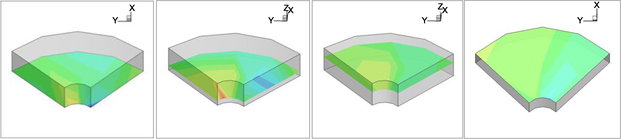
Figure 8. Contour plots of the velocity “w” at four heights for group 2-05.

Figure 9. Contour plots of the velocity “w” at three rings (3 m, 6 m, 9 m) for group 2-05.

Figure 10. Contour plots of the velocity “w” at five angles (side views) for group 2-05.
While the first two sets showed reasonable flow patterns, the contour plots of test set three did not show a shape of the plume. Meanwhile, paired two-sample t-test between test set three and test set two indicated significant differences between the two. This might be due to the variation of the background wind since the background wind and fan flow velocities were not measured simultaneously. Since only one group of test was done for the test set three, further experiments should be conducted to justify this method.
3.3. Plume Modeling and Visualization by CFD
The CFD modeling was conducted for the given boundary condition specified in Table 2 and Table 3. Upon obtaining the CFP outputs, paired two-sample t-test was used to test the difference between the CFD simulation and the field measurement. The results showed significant differences for comparing the model outputs in three velocities (u, v, w) with all groups’ measurements of the velocities. While the CFD model produced velocities in much smaller magnitude, it showed a similar flow direction, shifting to the left. The top-view of the plume at 0.3 m above the ground and the computational meshes modeled by FloEFD is presented in Figure 11.
The contour of the CFD model also provided similar velocity profile as illustrated by the TECPLOT, but with a smaller magnitude. As an example, Figure 12 shows left side view of the CFD contour plot.
3.4. Plume Shape Observation and Prediction
In this research, the plume shape is defined by the plume depth, width and rise. Examination of the plume shape was started with identification of the plume depth where the significant lifting starts. Based upon filed observations, the plume depth is defined as following: when the plume lifting velocity, w, increased alone the “x” direction to a point where it started decreasing, the distance x at this point was defined as the plume depth. To quantify this depth, the first two sets of “w” data were sorted from the smallest to largest and each data was ranked. After data sorting and ranking it was discovered that, like what Figure 12 has shown, the maximum of “w” appeared at the lower left part (x = 2.10 - 3.00 m, y = 0.00 - 2.14 m, z = 0.30 - 1.22 m) on the first ring, followed by points at the center (x = 8.3 m, y = 3.49 m, z = 1.22 m) on the second ring. On the third

Figure 11. Top-view of CFD modeled contour plot of 3D velocities at 0.3 m above the ground.

Figure 12. Side view of the contour plot of the velocity “w” modeled by the CFD.
ring, the biggest “w” appeared at the upper left part (x= 10.49 - 13.83 m, y = 5.81 - 10.72 m, z = 3.05 - 4.88 m), but these points had smaller w’s as compared to the first two rings. This suggests that at 3 m away from the fan, there was a strong lifting momentum; at around 9 m away from the fan, the lifting momentum was still big, but not as strong as at the 3 m ring.
Combining the data examination with the plots visualization, it was discovered that the plume depth was approximately 9 m away from the fan where the plume started to lift.
Similar method was used to examine the plume width and it was discovered that the plume width was about ±6 m.
For plume rise examination, the filed measurement was conducted with the furthest distance at 15 m and top height at 4.88 m. The field smoke test indicated that the plume went beyond 15 m away from fan and rose over 4.88 m. Limitation of the measurement height and distance prevent a numerical development of the plume rise at this time. Further experiment is planned to extend field measurement scope. Moreover, further CFD modeling will be conducted with different fan operation conditions examine ventilation rate impact on the plume field, and to calibrate the CFD output such that this modeling approach may be used to predict full scale of plume lifting the dispersion.
4. Summary and Conclusion
In this research, a combination of theoretical and field study was conducted to measure and simulate the plum rise and shape of air flow from a ventilation fan. The theoretical modeling of the plume shape was conducted using a commercial Computational Fluid Dynamics (CFD) package named FloEFD; the field measurements of the plume field was conducted using five 3D ultrasonic anemometers to simultaneously measure the air flow in the plume at various locations. The TECPLOT package was used to visualize the plume flow field based upon anemometer measurements. While the plume shapes were found to be left- shifted by the CFD model and TECPLOT visualization, the magnitudes of the 3D wind velocities from field measurement were found to be significantly larger than those from CFD model. The plume field measurements indicated that the plume of a 0.6 m (24-inch) ventilation fan had a depth about 9 m, a width about ±6 m, and a rise (lifting) beyond the highest measurement point, 4.88 m (16 ft). Further filed data collection is needed to extend measurement height to capture the true plume lifting height.
Acknowledgements
This study was supported in part by NSF CAREER Award No. CBET-0954673 and USDA NIFA Higher Education Challenger Grant Program 2013-70003-20929. Help from Roberto Munillia, Steven Badawi, Di Hu and Qianfeng Li for testing setup construction and field data collection is also thankfully acknowledged.
Cite this paper
Ying, M.Q., Wang-Li, L., Stikeleather, L.F. and Edwards, J. (2017) Measurements and Visualization of the Fluid Field of the Plume from an Animal Housing Ventilation Fan. Journal of Environmental Protection, 8, 1296-1311. https://doi.org/10.4236/jep.2017.811080
References
- 1. USDA/NASS (2005) Livestock and Poultry-Production and Value 2004 Summary. U.S. Department of Agriculture (USDA), National Agricultural Statistics Service (NASS), Washington, DC.
- 2. Heber, A.J., Bogan, W., Ni, J.Q., Lim, T.T., Ramirez-Dorronsoro, J.C., Cortus, E.L., Diehl, C.A., Hanni, S.M., Xiao, C., Casey, K.D., Gooch, C.A., Jacobson, L.D., Kozel, J.A., Mitloehner, F.M., Ndgwa, P.M., Rpbarge, W.P., Wang, L. and Zhang, R (2008) The Nation Air Emisison Monitoring Study: Overview of Barn Sources. Presented at ILES VIII, Publisher, City.
- 3. National Research Council (2003) Air Emissions from Animal Feeding Operations: Current Knowledge, Future Needs. The National Academies Press, Washington DC.
- 4. Wang, K., Kilic, I., Li, Q.F., Wang-Li, L.J., Bogan, W.L. and Heber, A.J. (2010) National 386 Air Emissions Monitoring Study: Emissions Data from Two Tunnel-Ventilated Layer Houses in North Carolina-Site NC2B. Final Report. Purdue University, West Lafayette.
- 5. Briggs, G.A. (1971) Plume Rise: A Recent Critical Review. Nuclear Safety, 12, 15-24.
- 6. Maes, G., Cosemans, G., Kretzschmar, J., Janssen, L. and Vantongerloo, J. (1995) Comparison of 6 Gaussian Dispersion Models Used for Regulatory Purposes in Different Countries of the Eu. International Journal of Environment and Pollution, 5, 734-747.
- 7. Singal, S.P., Gera, B.S. and Pahwa, D.R. (1994) Application of Sodar to Air Pollution Meteorology. International Journal of Remote Sensing, 15, 427-441. https://doi.org/10.1080/01431169408954084
- 8. Yadigaroglu, G., and Munera, H.A. (1987) Transport of Pollutants—Summary Review of Physical Dispersion Models. Nuclear Technology, 77, 125-149. https://doi.org/10.13182/NT87-A33979
- 9. Awasthi, S., Khare, M. and Gargava, P. (2006) General Plume Dispersion Model (GPDM) for Point Source Emission. Environmental Modeling & Assessment, 11, 267-276. https://doi.org/10.1007/s10666-006-9041-y
- 10. Hiscox, A.L., Miller, D.R., Holmén, B.A., Yang, W. and Wang, J. (2008) Near-Field Dust Exposure from Cotton Field Tilling and Harvesting. Journal of Environmental Quality, 37, 551-556. https://doi.org/10.2134/jeq2006.0408
- 11. Cooper, C.D. and Alley, F.C. (2002) Air Pollution Control: A Design Approach. 3rd Edition, Waveland Press, Prospect Heights.
- 12. Holmes, N.S. and Morawska, L. (2006) A Review of Dispersion Modeling and Its Application to the Dispersion of Particles: An Overview of Different Dispersion Models Available. Atmospheric Environment, 40, 5902-5928.
- 13. Wendt, J.F. and Anderson, J.D. (2009) Basic Philosophy of CFD. In: Computational Fluid Dynamics: An Introduction, Spinger Verlag, Berlin, Heidelberg, 5-8.
- 14. Alic, G., Sirok, B. and Hocevar, M. (2010) Method for Modifying Axial Fan’s Guard Grill and Its Impact on Operating Characteristics. Forsch Ingenieurwes, 74, 87-98. https://doi.org/10.1007/s10010-010-0118-z
- 15. Gates, R.S., Casey, K.D., Xin, H., Wheeler, E.E. and Simmons, J.D. (2004) Fan Assessment Numeration System (FANS) Design and Calibration Specifications. Transactions of ASAE, 47, 1709-1715. https://doi.org/10.13031/2013.17613
- 16. Wang, X., Chen, R. and Zhou, Y. (2011) The Flow Field Analysis and Optimization of Diagonal Flow Fan Based on CFD. Advanced Materials Research, 201-203, 2657-2660. https://doi.org/10.4028/http://www.scientific.net/AMR.201-203.2657
- 17. Quinn, A.D., Wilson, M., Reynolds, A.M., Couling, S.B. and Hoxey, R.P. (2001) Modeling the Dispersion of Aerial Pollutants from Agricultural Buildings—An Evaluation of Computational Fluid Dynamics (CFD). Computers and Electronics in Agriculture, 30, 219-235.
- 18. Tecplot, Inc. (2011) Tecplot 360 User’s Manual. Tecplot, Inc., Bellevue.
- 19. Kun, L., Zhe, W., Han, R. and Ren, Z. (2011) The Numerical Simulation of Directional Solidification Process Temperature Field for Large-Scale Frustum of a Cone Ingot. Manufacturing Process Technology, 189-193, 1476-1481.
- 20. Gong, Y., Zhang, Y., Li, H. and Wang, W. (2009) A Study on Airflow Field of Super-High Speed Pectination Grinding Wheel Based on PIV. Advances in Abrasive Technology, 389-390, 332-337.
- 21. Muramalla, K., Chen, Y. and Hechanova, A. (2005) Simulation and Optimization of Homogeneous Decomposition of Sulfur Trioxide Gas on a Catalytic Surface. Heat Transfer Division of the American Society of Mechanical Engineers, 376, 201-207.
- 22. Turner, D.B. (1994) Workbook of Atmospheric Dispersion Estimates: An Introduction to Dispersion Modeling. 2nd Edition, CRC Press, Boca Raton.
- 23. Pasquill, F. (1961) The Estimation of the Dispersion of Windborne Material. Meteorology Magazine, 90, 33-40.
- 24. Gifford, F.A. (1976) Consequences of Effluent Releases. Nuclear Safety, 17, 68-86.
- 25. Linacre, E. and Geerts, B. (1999) Roughness Length. The University of Wyoming, 358 WY. http://www.das.uwyo.edu/~geerts/cwx/notes/chap14/roughness.html