Journal of Environmental Protection
Vol.07 No.06(2016), Article ID:66337,12 pages
10.4236/jep.2016.76072
Life-Cycle Analysis of Bio-Ethanol Fuel Emissions of Transportation Vehicles in Greater Houston Area
Raghava Kommalapati1,2*, Shahzeb Sheikh1, Hongbo Du1, Ziaul Huque1,3
1Center for Energy & Environmental Sustainability, Prairie View A&M University, Prairie View, USA
2Department of Civil & Environmental Engineering, Prairie View A&M University, Prairie View, USA
3Department of Mechanical Engineering, Prairie View A&M University, Prairie View, USA

Copyright © 2016 by authors and Scientific Research Publishing Inc.
This work is licensed under the Creative Commons Attribution International License (CC BY).
http://creativecommons.org/licenses/by/4.0/


Received 30 March 2016; accepted 8 May 2016; published 11 May 2016
ABSTRACT
Study is conducted on the life cycle assessment of bio-ethanol used for transportation vehicles and their emissions. The emissions that are analyzed include greenhouse gases, volatile organic compounds, sulfur oxide, carbon monoxide, nitrous oxide, particulate matter with the size less than 10 and 2.5 microns. Furthermore, various blends of bio-ethanol and gasoline are studied to learn about the impacts of higher blend on emissions. The Greenhouse Gases, Regulated Emissions, and Energy Use in Transportation (GREET) model software are used to simulate for emissions. The research analyzes two pathways of emissions: Well-to-Pump and Pump-to-Vehicle analyses. It is found that the fuel cell vehicles using 100% bio-ethanol have shown the most reduction in the amount of all the pollutants from the Pump-to-Vehicle emission analysis. The Well-to-Pump analysis shows that only greenhouse gases (GHGs) reduce with higher blends of bio-ethanol. All other pollutants VOC, CO, NOx, SOx, PM10 and PM2.5 emissions increase with the higher blending ratios. The Pump-to-Vehicle analysis shows that all the pollutant emissions reduce with the percentage increase of bio-ethanol in the fuel blends.
Keywords:
Life Cycle Assessment, Bio-Ethanol, Greenhouse Gases Emissions, Pollutant Emissions

1. Introduction
Transportation vehicles are mainly run on liquid fossil fuel, gasoline and diesel. As the population grows, the demand of transportation vehicles increases and leads to the high usage of fossil fuels. Future prediction on the usage of vehicles suggests that developing countries are expected to account for 52% of the total worldwide mobility in 2050 with 54,545 billion passenger kilometer (pkm) (versus 8562 billion pkm or 37% in 1990) [1] . According to one comparative study of USA and Japan, transportation accounts for more than one forth (the contribution is higher in USA) of the total energy consumption, and road transportation vehicles account for more than 80% (the contribution is higher in Japan) of the total transportation energy consumption [2] . There are quite a few issues with the increasing demand of fuel in transportation sector. It includes non-renewable energy issues, decline of energy resources for future use, greenhouse gases (GHGs) emissions responsible for climate change and other pollutants in the environment.
The reliance of transport on fossil fuel appears to be causing long-term damage to the climate [3] . Many adverse effects of high fuel consumption by transportation vehicles are predicted. According to IPCC (Intergovernmental Panel on Climate Change), it is high likely for the global temperature to rise between 1.4˚C and 5.8˚C which will result in extreme weather events and a rise in sea levels [3] . Furthermore, burning of fuel by vehicles emits other pollutants which are responsible for the damage of our ozone level ultimately causing health problems in addition to global warming. The primary component responsible for global warming is greenhouse gases. Under the six illustrative emission scenarios used by the IPCC, the CO2 global level was predicted to increase over the next century from 369 parts per million, to between 540 and 970 parts per million [3] . Some statistics showed the CO2 emissions per transport sector: road transport (65%), rail, domestic Aviation & waterways (23%), international aviation (5%), international shipping (7%) [3] . One study confirmed that 60% - 65% of life-cycle greenhouse gases are CO2 exhaust emissions from petro-engine cars [4] . Another source predicted that carbon emissions from passenger transport maybe increase worldwide from 0.8GtC (gigatonnes carbon) in 1990 to 2.7 GtC in 2050 [1] .
Use of bio-fuels is one of the best possible alternative solutions available to solve the issue. Bio-fuels are renewable sources of energy which can be produced from various resources such as plants and wastes. In the US, the first generation bio-fuel, mainly bio-ethanol is used in transportation. Use of bio-ethanol in vehicles not only limits the dependency on fossil fuel, but also helps in lowering greenhouse gases emissions. Also, air pollutant emissions from vehicle tailpipes that are really harmful to human health will be lowered with bio-fuels [5] . Bio-ethanol can be used in two ways: direct usage in the vehicles and in the form a blends of various volume of petro-fuel to bio-ethanol.
Houston, Texas is considered one of the most polluted cities due to its transportation and industrial emissions. The increasing emissions of VOCs, NOx and other criteria pollutants are affecting the air quality by acting as precursors of ground ozone production. Thus, the use of bio-fuels will have an improving impact on the air quality of Houston. The objective of this study is to analyze the life cycle assessment of bio-ethanol from corn feedstock. Various emissions of gases will be analyzed including GHGs, VOC, CO, NOx, SOx, PM10, PM2.5 from the production of fuels (Feedstock + Fuel) and vehicle usage. Furthermore, different blends of petro-fuel and bio-ethanol by volume are simulated, and higher blends trends are analyzed. The GREET (Greenhouse gases, Regulated Emissions, and Energy use in Transportation) Fuel-cycle software is used to simulate for emissions in kg/day using VMT (vehicle miles travelled) report of Houston, TX.
2. Methodology
2.1. GREET Model Software
The GREET model software is used to simulate fuel cycle for the transportation vehicles. The software is developed by Argonne National Lab [6] . It basically analyzes energy use, emissions of GHGs and other criteria pollutants for vehicle/fuel system. The software is Excel based with various screens for inputs and choosing fuel pathways. Brief explanation about the software is discussed below.
First, input sheets are available to guide users in GREET Model. It consists of key variables for various Well-to-Pump (WTP) and Pump-to-Vehicle (PTV) scenarios, and identifies key parametric assumptions for GREET simulations [7] . The GREETGUI is the front end user interface, which helps in setting parameters for the fuel pathways to be simulated by GREET. Next, GREET model currently analyzes light duty vehicles:
・ Passenger cars (PC)
・ Light-duty trucks 1 (LDT1) with a gross vehicle weight (GVW) less than 6000 lbs
・ Light-duty trucks 2 (LDT2) with a GVW between 6000 and 8500 lbs [7] .
There are more than 70 vehicle/fuel pathways available to simulate in GREET. Baseline vehicles in GREET are spark ignition (SI) vehicles fueled with CG (conventional gasoline) and/or RFG (reformulated gasoline), and CIDI vehicles fueled with CD (conventional diesel) and/or LSD (conventional diesel) [7] . The sheets, Car TS, LDT1_TS and LDT2_TS present with the parameters for calculations of passenger cars, LDT1 vehicles and LDT2 vehicles respectively. Nine vehicle technologies are available in GREET such as SI vehicles (e.g., LPG, E85, and others), Spark-ignition direct-injection (SIDI) vehicles (e.g., gasoline, E90, and others), Grid- independent (GI) SI HEVs (e.g., gasoline, CNG, and others), Fuel cell vehicles (FCVs) (e.g., H2, ethanol, and others) [7] .
2.2. Fuel Blends and Engines Types
Various fuel blends of petrol-fuel and bio-ethanol by volume are analyzed and compared with the gasoline. Fuel blends includes E0, E10 (10% ethanol and 90% gasoline), E85 and E100. Next, the vehicle engines types that are chosen are spark ignition (SI) engine, flexible fuel vehicle (FFV) including dedicated bio-ethanol type, and fuel cell vehicle (FCV).
2.3. Targeted Years
2011, 2014 and 2017 are the years that are selected for running simulations. The base year for GREET software is taken as 2006, due to the availability of vehicle model data.
2.4 VMT Development
VMT (vehicle miles travelled) reports of Houston for the 2002-2013 years are available from the website database of the U.S. Department of Transportation/Federal Highway Administration [8] [9] . However, 2014 and 2017 VMT reports aren’t available. The trend of miles traveled for the years 2015 and 2018 is considered with the economic conditions, the rise in population and vehicle demand in Houston [10] [11] .
2.5. GREET Model Simulations
After determining parameters and obtaining VMT data for Houston, life cycle assessment of bio-ethanol emissions is simulated for the selected fuel/vehicle pathways and targeted years. First, simulations for the 2011 year are performed. The bio-ethanol blend levels consist of low level blend (5% - 25% by volume with gasoline), high level blend (50% - 90% by volume with gasoline) and 100% ethanol for fuel cell vehicles (FCV). In the following sections simulations are carried out for E0, E10, E85 and E100 and for the years of 2014 and 2017. After obtaining the data in the form of excel sheets. The data is converted from Btu/mile to kg/day using VMT of Houston. Graphs and percentage analysis are performed as well.
3. Results and Discussion
3.1. Daily Travel Model VMT
The data in Table 1 is developed after finding the ratio of different vehicle types and performing required calculations for VMT of passenger cars, LDT1 and LDT2. It can be seen that passenger cars run more miles than LDT1 and LDT2 vehicles. Also, the trend of miles traveled seems to be increasing year by year as expected due to rise in population and vehicle demand.
3.2. Emission Analysis
The life cycle assessment of bio-ethanol emissions performed by GREET model simulation consists of two stages of fuel cycle: Well-to-Pump and Pump-to-Vehicle emissions analysis. First, Well-to-Pump analysis focuses on the feedstock and fuel selections. Feedstock stage addresses the energy use or emissions released in gathering raw materials (land use, distribution etc.). Fuel stage analyses the emissions in developing the specific fuel such as E10, E85 etc. Next, Pump-to-Vehicle emissions analysis focuses on studying the pollutant emissions from vehicle operation. The calculated results are listed in Tables 2-4 for each bio-ethanol fuel blend, vehicle engine type and year. Furthermore, the emissions plots are created to show percentage reduction. The negative percentage in reduction shows the increase in the particular gas emissions.

Table 1. VMT of Houston by vehicle classifications and analysis years.
Table 2. Well-to-pump 2011, 2014, 2017 daily total emissions of pollutants in kg/day for passenger cars.
Table 3. Well-to-pump 2011, 2014, 2017 daily total emissions of pollutants in kg/day for LDT1.
Table 4. Well-to-pump 2011, 2014, 2017 daily total emissions of pollutants in kg/day for LDT2.
3.3 Well-to-Pump Emissions Analysis
The Well-to-Pump analysis refers to the emissions of pollutants from the production of fuel blends. Tables 2-4 list the simulation results of Well-to-Pump emission analysis for year 2011, 2014, and 2017 of passenger cars, LDT1 and LDT2 vehicles after incorporating the VMT results for Houston. The results in Table 2 show that GHG emissions reduce with the increasing blend ratio of bio-ethanol in gasoline. Other pollutant emissions such as VOC, NOx, PM10, PM2.5, and SOx increase as the production of higher bio-ethanol blends ratio until E85. However, 100% bio-ethanol fuel emits less VOC, NOx, PM10, PM2.5, and SOx pollutants than E85. Comparison between different targeted years under the same bio-ethanol blend ratio, GHG emissions with E100 are negative for the target years 2014 and 2017, indicating the more achievement of GHGs reduction with the technology development. Other pollutant emissions similarly demonstrate the greater reductions for future years. Moreover, the simulation results for the LDT1 and LDT2 vehicles resemble those of the passenger cars in terms of the reducing and increasing trends for all the pollutant emissions.
Figure 1 shows the percentage reductions of pollutant emissions at the Well-to-Pump stage for the target year 2017. The negative percentage in reduction shows the increase in the particular pollutant emissions. The results show that only GHGs reduce when using higher blends of bio-ethanol in feeding fuels. Reduction of 5%, 84% and 111% GHGs achieve when producing E10, E85 and E100 fuel blends respectively. However, the other pollutants VOC, SOx, NOx, CO, PM10 and PM2.5 have negative percentage with emission increased for E10, E85 and E100. In more details, the other pollutant emissions demonstrate some reductions at E100 from those at E85. Following the trends of increasing and reducing emissions with passenger cars, LDT1 and LDT2 vehicles show the similar percentage plots for all the pollutant emissions. Figure 2 and Figure 3 illustrate the percentage reductions of LDT1 and LDT2 which indicate similar trend.
3.4. Pump-to-Vehicle Emissions Analysis
The Pump-to-Vehicle emission analysis refers to the pollutant emissions from the use of fuel blends by different vehicle engine types. Houston’s VMT report is used to determine the emissions in kg/day. The Pump-to-Vehicle is crucial in a sense that it accounts for more than half of the total emissions starting from wells.
Passenger Cars are the most driven vehicles in Houston area. Thus, they are responsible for the most emissions of pollutants. Passenger cars are simulated for engines including SI, FFV, FFV-Dedicated and FCV and various fuel blends. Tables 5-7 list the emissions of pollutants in kg/day for passenger cars, LDT1 and LDT2 vehicles respectively. Moreover, 2011, 2014, and 2017 years are simulated as proposed. Figures 4-6 show the percentage reduction of emissions for passenger cars, LDT1 and LDT2 vehicles respectively.

Figure 1. Well-to-pump 2017 percentage reductions of emissions for passenger cars.
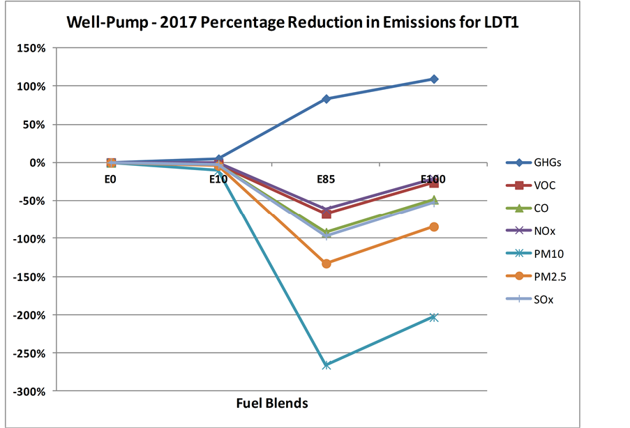
Figure 2. Well-to-pump 2017 percentage reductions of emissions for LDT1.

Figure 3. Well-to-pump 2017 percentage reductions of emissions for LDT2.
Table 5. Pump-to-vehicle 2011, 2014, 2017 daily total emissions of pollutants in kg/day for passenger cars.
Table 6. Pump-to-vehicle 2011, 2014, 2017 daily total emissions of pollutants in kg/day for LDT1.
Table 7. Pump-to-vehicle 2011, 2014, 2017 daily total emissions of pollutants in kg/day for LDT2.
![]()
Figure 4. Pump-to-vehicle 2017 percentage reductions of emissions for passenger cars.
![]()
Figure 5. Pump-to-vehicle 2017 percentage reductions of emissions for LDT1.
![]()
Figure 6. Pump-to-vehicle 2017 percentage reductions of emissions for LDT2.
The GHGs are the major emitted gases of all the targeted pollutants. As the higher blends are introduced, the GHGs, VOC, CO, NOx, PM10, and PM2.5 seem to be reduced at a very slow rate till E85. The VOC emissions for E100 reduce about 73% for all the target years. The CO and NOx emissions for E100 reduce about 80% for the different target years. The PM10 and PM2.5 emissions for E100 fueled into FCV reduce about 43% and 66% for the different target years respectively. The SOx emissions reduce with the increase of bio-ethanol blend ratio and reach 0 at E100. Furthermore, similar trends in percentage reduction of all the pollutants are obtained for LDT1 and LDT2 vehicles.
4. Conclusions
The life cycle emissions of GHGs, VOC, CO, NOx, SOx, PM10, and PM2.5 for bio-ethanol fuel blends with gasoline in Houston market are studied. Life cycle assessment according to two modes Well-to-Pump and Pump-to-Vehicle is simulated using GREET model.
It is determined that the pollutant emissions not only depend on the fuel type, but also the type of vehicle engine. First, the Well-to-Pump analysis shows that only GHGs emissions reduce with the higher bio-ethanol fuel blend. However, all other pollutants VOC, NOx, CO SOx, PM10 and PM2.5 pollutant emissions increase for increasing bio-ethanol fuels blend ratio. All other pollutants, VOC, NOx, SOx, and PM10 demonstrate the increasing emissions until E85 blending ratio. 100% bio-ethanol fuel fueled into FCV cars emits less VOC, NOx, PM10, PM2.5, and SOx pollutants than E85 used in FFV cars. Next, Pump-to-Vehicle emissions analysis provides a positive relationship between emissions reduction and higher blends of bio-ethanol usage in vehicles. The 100% bio-ethanol fuel remains the best options to use in transportation vehicles because it reduces the emissions of all the pollutants for the FCV vehicles discussed. All the targeted years for simulations follow the same trend for emissions.
Thus, the research concludes that FCV using E100 is the best option to improve the air quality of Houston. There may be several factors which can bring hurdles in implementing FCV with E100 in the market. These factors are probably the increased cost of manufacturing fuel cell vehicle, energy density problem with the bio-ethanol fuel, land consumption to produce bio-ethanol fuel and low freezing point of bio-ethanol which may not be suitable for winter time.
Acknowledgements
This research was supported by the National Science Foundation (NSF) through the Center for Energy and Environmental Sustainability (CEES), a CREST Center award #1036593.
Cite this paper
Raghava Kommalapati,Shahzeb Sheikh,Hongbo Du,Ziaul Huque, (2016) Life-Cycle Analysis of Bio-Ethanol Fuel Emissions of Transportation Vehicles in Greater Houston Area. Journal of Environmental Protection,07,793-804. doi: 10.4236/jep.2016.76072
References
- 1. Poudenx, P. (2008) The Effect of Transportation Policies on Energy Consumption and Greenhouse Gas Emission from Urban Passenger Transportation. Transportation Research Part A, 42, 901-909. http://dx.doi.org/10.1016/j.tra.2008.01.013
- 2. Jia, S., Peng, H., Liu, S. and Zhang, X. (2009) Review of Transportation and Energy Consumption Related Research. Journal of Transportation Systems Engineering and Information Technology, 9, 6-14. http://dx.doi.org/10.1016/S1570-6672(08)60061-6
- 3. Chapman, L. (2007) Transport and Climate Change: A Review. Journal of Transport Geography, 15, 354-367. http://dx.doi.org/10.1016/j.jtrangeo.2006.11.008
- 4. Colvile, R.N., Hutchinson, E.J., Mindell, J.S. and Warren, R.F. (2001) The Transport Sector as a Source of Air Pollution. Atmospheric Environment, 35, 1537-1565. http://dx.doi.org/10.1016/S1352-2310(00)00551-3
- 5. Wu, M., Wu, Y. and Wang, M. (2006) Energy and Emission Benefits of Alternative Transportation Liquid Fuels Derived from Swithgrass: A Fuel Life Cycle Assessment. Biotechnology Progress, 4, 1012-1024. http://dx.doi.org/10.1021/bp050371p
- 6. (2015) GREET Model Software. Energy System, Argonne National Laboratory. https://greet.es.anl.gov/
- 7. Wang, M., Wu, Y. and Elgowainy, A. (2007) Operating Manual for GREET Version 1.7. Center for Transportation Research, Energy Systems Division, Argonne National Laboratory
- 8. Federal Highway Administration (FHWA) (2009) Table HM-71-Highway Statistics 2008-FHWA. https://www.fhwa.dot.gov/policyinformation/statistics/2008/hm71.cfm
- 9. Federal Highway Administration (FHWA) (2002) Highway Statistics 2002—URBANIZED AREAS—2002—Table HM-71. https://www.fhwa.dot.gov/policy/ohim/hs02/hm71.cfm
- 10. Lubertino, G., Gao, D., Smith, C., Slyke, C.V. and Whitworth, S. (2009) Texas Houston-Galveston Area Council. Transportation Development and Production of On-Road Mobile Source Reasonable Further Progress Emission Inventories for the Years 2002, 2008, 2011, 2014, 2017, 2018, and 2019. Houston-Galveston Area Council, Texas Commission on Environmental Quality.
- 11. Texas Transportation Institute (TTI) (2009) 2008 CERR On-Road Mobile Source CERR Emissions Inventories for the HGB Area. Transportation Modeling Program.
NOTES
![]()
*Corresponding author.