Journal of Environmental Protection
Vol.4 No.5A(2013), Article ID:31896,16 pages DOI:10.4236/jep.2013.45A004
Identification of Contaminant Source Characteristics and Monitoring Network Design in Groundwater Aquifers: An Overview
![]()
1Discipline of Civil and Environmental Engineering, School of Engineering and Physical Sciences, James Cook University, Townsville, Australia; 2Cooperative Research Centre for Contamination Assessment and Remediation of Environment, Mawson Lakes, Australia.
Email: mahsa.amirabdollahian@jcu.edu.au, bithin.datta@jcu.edu.au
Copyright © 2013 Mahsa Amirabdollahian, Bithin Datta. This is an open access article distributed under the Creative Commons Attribution License, which permits unrestricted use, distribution, and reproduction in any medium, provided the original work is properly cited.
Received March 15th, 2013; revised April 17th, 2013; accepted May 15th, 2013
Keywords: Pollution Detection; Aquifer Contamination; Groundwater; Source Identification; Monitoring Network Design
ABSTRACT
The groundwater system is often polluted by different sources of contamination where the sources are difficult to detect. The presence of contamination in groundwater poses significant challenges to its delineation and quantification. The remediation of a contaminated site requires an optimal decision making system to identify the pollutant source characteristics accurately and efficiently. The source characteristics are generally identified using contaminant concentration measurements from arbitrary or planned monitoring locations. To effectively characterize the sources of pollution, the monitoring locations should be selected appropriately. An efficient monitoring network will result in satisfactory characterization of contaminant sources. On the other hand, an appropriate design of monitoring network requires reliable source characteristics. A coupled iterative sequential source identification and dynamic monitoring network design, improves substantially the accuracy of source identification model. This paper reviews different source identification and monitoring network design methods in groundwater contaminant sites. Further, the models for sequential integration of these two models are presented. The effective integration of source identification and dedicated monitoring network design models, distributed sources, parameter uncertainty, and pollutant geo-chemistry are some of the issues which need to be addressed in efficient, accurate and widely applicable methodologies for identification of unknown pollutant sources in contaminated aquifers.
1. Introduction
Groundwater is the major potable, agricultural and industrial source of water. In 2003, it was estimated that groundwater possess approximately 50% of potable water supplies, 40% of industrial water demand, and 20% of water used for irrigation [1]. To ensure the water security, the sustainability of groundwater resources is vital. Due to industrial revolution together with the lack of appreciation of chemicals and their potential impact on the land and water bodies, groundwater is subjected to various sources of contamination. The presence of contamination in groundwater poses significant challenges to its delineation and quantification. Leakage from chemical and petrochemical distribution infrastructures, e.g. pipelines and waste water collection systems such as septic tanks and urban sewage channels and pipelines are few real life examples of unknown subsurface contamination. Further, products of mining activities and industrial complexes, which are stored on or underground without any provision to control the seepage of contamination into the ground, have been two of the most challenging and difficult problems associated with contamination management during the past 100 years.
The contamination in underground water may remain undetected for significant period of time. The first signs of the presence of contaminate underground water may be detected from the water extracted from current extraction wells. Change in the surface water quality, like rivers or lakes, possibly stems from presence of contamination in underground water. Awareness of groundwater pollution has grown in last two decades. The spread of pollution in underground water raised the necessity to develop efficient techniques for remediation of contaminated aquifer. The effectiveness of a remediation strategy depends on how efficiently the contamination source characteristics are identified. Accurate identification of the contaminant sources and reconstructing their release history plays an important role in modelling of subsurface flow and transport processes, and help to reduce the long-term remedial costs.
Accurate and efficient characterization of unknown contamination sources in the groundwater system is the critical first step in the process of controlling and remediation of subsurface pollution. This problem is more complex for subsurface pollution, as pollution of surface water bodies are relatively easier to detect. Some of the available methodologies for groundwater pollution source identification are reviewed here. However, it needs to be emphasised that often the efficiency of source identification depends on the availability and reliability of concentration field measurements, and hydro-geologic information. Therefore a designed monitoring network for collection of field geochemical measurements can help to improve the efficiency of source identification. The iterative use of source identification modelsand a sequentially design monitoring network for source identification can be integrated in an efficient source characterization methodology. This aspect is also reviewed here.
The pollutant source characteristics which need to be identified include:
• The spatial locations of sources.
• The activity duration of sources which identifies when the sources became active
• The injection rate of the pollutant sources which specifies the contaminant flux released from each source as a function of time.
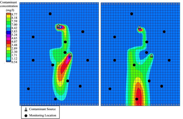
The identification of unknown pollutant sources and the propagation of contaminants in underground water are mostly inferred from the available concentration measurements at the site. Figure 1 shows a polluted aquifer. In this figure the location of two active pollutant sources, the propagation of contaminant in aquifer as well as available monitoring locations, are shown. In Figures 1(a) and (b), the contours show the contaminate concentration values after 250 and 900 days after start of source activity.
Mainly source identification includes a forward simulation problem, like groundwater flow and pollutant transport model, which is used to estimate phenomena or
 (a) (b)
Figure 1. Contaminant aquifer: (a) After 250 days of source activation; (b) After 900 days of source activation.
predict future scenario. The estimated values are then compared with observed values. Effective selection of observation points plays a critical role in source identification model. An improper monitoring network will result in waste of time and money for site data collection, and may result in misleading optimal source identification results. This is because multiple source characteristic scenarios might fit the observed data which do not adequately defining the actual contaminant characteristics.
Figure 1 also shows the monitoring network. In this figure, the monitoring locations were selected arbitrary without having any prior information about the sources of contamination. It can be seen that many of selected locations do not adequately catch the pollutant plume. Furthermore, the temporal schedule of collecting data is very important. The monitoring wells which are located far from the active sources are also useful in later times, as these capture later part of the pollutant plume. However, the ones which are located near active sources play important role in capturing the plume soon after the source activities begin. Also, any concentration measurement location is of little use when the contaminate plume is not captured at that monitoring location. Selection of an appropriate monitoring network, and an implementation of effective monitoring schedule to obtain information about the sources of contamination and propagation of the pollutant plume, are vital for efficient and accurate source identification.
An efficient monitoring network will result in satisfactory characterization of contaminant sources. On the other hand, an appropriate design of monitoring network requires reliable source characteristics. A coupled iterative sequential source identification and dynamic monitoring network design, can improve substantially the accuracy of source identification model [2].
In the absence of an efficient monitoring network, preferably designed to improve the source identification process, errors in the available concentration data pertaining to the contaminated site will impose uncertainty to the mathematical and numerical methods for solving the source identification problem. In addition to this source of uncertainty, lack of hydro-geological parameter information results in uncertain groundwater and solute transport modelling. The most important first step in ensuring the long term environmental sustainability of groundwater resources is the effective control of groundwater contamination. The most important first step in subsurface control and remediation is an accurate identification of unknown sources.
This study aims to present a comprehensive review of previous published researches on the contaminant source identification models. In this framework, first the main issues needed to be considered and addressed in this area are presented. It is followed by a review of source identification and monitoring network design methodologies. An integration of source identification and monitoring network design is discussed in the next section. Lastly, some of the issues which need future attention in this area are presented.
2. Main Issues
The pollutant source identification problem can be treated as an inverse problem. The main objective of existing methodologies of source identification is to minimize the difference between the observed values and simulated values of contaminant concentration at designed monitoring locations. The contaminant concentrations are simulated using estimated source characteristics. In general, an inverse problem is considered well posed if following conditions are satisfied [3]:
• A solution exists• The solution is unique, and
• The solution is stable.
Since the propagation of contaminant started from one or more sources, thus there exists a solution for the inverse source identification model. However, unlike forward modelling, it may not have unique solution and may lack of stability. Therefore the ground water pollutant source characterization is often considered an illposed inverse problem.
In general, an inverse modelling of any physical system requires great computational effort. Availability of adequate field measurement and parameter values are critical to the inverse source identification procedure. However, acquiring data is a very cost and time consuming task. Thus the unknown groundwater pollution source identification is often characterized by very little information and is considered complex or not sufficiently known. Nonlinearity in underground flow and pollutant transport governing equations, increase the complexity of this problem. Solving the finite difference form of flow and transport equations, the aquifer should be discretised. To guarantee the stability of utilized numerical methods, fine discretisation is required, which will result in huge number of cells especially in real aquifers. This also increases the computational complexity of source identification problem.
The source identification model requires an accurate flow and transport model to estimate the contaminant concentration distribution in aquifer. The lack of parameter information results in uncertain groundwater and solute transport model. These uncertainties arise from a) human and machine imprecision in measurements; b) spatial variability of soil hydraulic properties as well as errors at un-sampled locations; c) use of parameter values measured in the laboratory for field conditions; d) “soft” quality information about the parameters based on subjective interpretation or expert judgment [4]. The solution of source identification model is highly sensitive to measurement errors either in the observation data or model parameters [5].
Mostly the only initial available information is the contaminant concentration in one or more arbitrary location of affected wells, and possibly some guesses about the location of sources. In some of the cases the contaminant source location is obvious from the available preliminary data. For the study areas in which extensive record of industrial activities, release or storage of pollutants are available, it may be possible to infer other characteristics of sources, like the start time of activation or release history. However, in most of the real life groundwater contamination cases there is not such comprehensive information available. The sources may be undetected for long period of time, or the pollutants are not accessible at extraction wells for an unknown period of time since the start of source activities. In such situations the source identification model should specify the source location, start time and release flux. The resulting number of variables requiring estimation makes the source identification model even more complex than before. In this situation the source characterization has to be undertaken by using measured information from a set of monitoring wells. The high degree of dependency on data collected from monitoring locations indicates the importance of an efficient monitoring network design model. A properly chosen monitoring network increases the accuracy of source identification model and decreases the total data collection costs. Figure 2 shows the errors in estimating the characteristics of contamination sources with and without incorporating measurement data from a designed monitoring network [2]. The feed-back data set shows the results when the integration of source identifycation and monitoring network design were utilized. As shown in Figure 2, the integration of a monitoring network and the source identification procedure, in general, results in increased efficiency of estimation.
The monitoring wells are selected based on the pollutant source characteristics, and the estimation transport of contamination. Therefore, the source identification
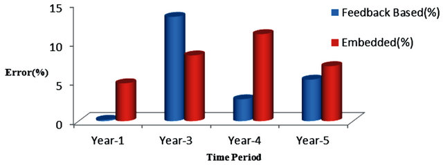
Figure 2. Error in estimation of source fluxes [2].
and monitoring network design should be addressed in a sequential manner [2]. In this framework, a real time monitoring network can be utilized to increase the accuracy of the source identification model.
3. Identification of Pollutant Source Characteristics
Identifying or characterizing unknown pollutant sources consist of answering three important questions regarding the contaminant sources.
• When was the contaminant released from the source? (Release history).
• Where is the contamination source? (Source location).
• At what concentration was the contaminant released from the source? (Source magnitude).
The contaminant transport process consists of three main phenomena of dispersion, advection and chemical reactions. The contaminant transport model represents an irreversible process. This makes an inverse modelling contamination transport an ill-posed problem. Ill-posed problems exhibit discontinuous dependence on data and high sensitivity to measurement errors. This problem is considered ill-posed since its solution does not satisfy following conditions: existence, uniqueness and stability. In the plume history problem, conditions of existence are assumed to be satisfied, since the plume had to be generated from somewhere. But the two remaining conditions are not satisfied [5].
The first approaches used to treat contaminant transport problems were stochastic ones. Gelhar [6] introduced new stochastic subsurface hydrology techniques. He examined the basic stochastic methods to treat flow and contaminant transport in naturally heterogeneous permeable earth materials. Using techniques that will overcome the problems of non-uniqueness and instability, new approaches which aim to solve the differential equations as inverse problem, were introduced. The random walk particle method [7,8], the quasi-reversibility technique [9], the minimum relative entropy method [10], the Bayesian theory and geostatistical techniques [11] and Genetic Algorithm (GA) [12,13], are some of these methods. Atmadja and Bagtzoglou [14] gives an overview on application of various inverse modelling techniques in pollution source identification problems.
Wagner [15] developed an inverse model for simultaneous parameter estimation and contaminant source characterization. A distributed source term was included as a parameter in a coupled two-dimensional groundwater flow and contaminant transport model. The source characteristics and model parameters were found using nonlinear maximum likelihood estimation. This model was able to consider both temporal and spatial contaminant release history. This model was found to be effective in numerical examples with exact knowledge of the model parameter zonation and a simple contaminant release history.
Due to similarity between heat and mass transport models and flow and contaminant transport ones, hydrodynamics can be used to overcome ill-posed problems in source identification models. Skaggs and Kabala [16] using the Tikhonov Regularization (TR), changed the ill-posed problem of contaminant source identification to a well-posed minimization problem. Using a one dimensional homogenous system the method evaluation was done incorporating error free and erroneous data. To generate erroneous data, a normal distributed random term was added to concentration observation values and aquifer parameters. Their results demonstrated that the accuracy of plume concentration is dependent on the accuracy of characterization of current plume and the extent to which plume was dissipated. Liu and Ball [17] tested [16]’s method at a low permeability site at Dover Air Force Base, Delaware. Skaggs and Kabala [9] applied more computationally efficient and easier to use method called Quasi-Reversibility (QR) to the previous problem. However, the results showed that the advantages of QR method come at the expense of accuracy. Skaggs and Kabala [18] used Monte Carlo numerical simulation to determine the ability of recovering various test functions by their proposed method.
An inverse problem approach was applied to the same problem as Skaggs and Kabala [16] by Woodbury and Ulrych [10]. They used a statistical inference method called Minimum Relative Entropy (MRE). Neupauer et al. [19] evaluated the relative effectiveness of TR and MRE methods in reconstructing the release history of conservative contaminant in one-dimensional domain. Snodgrass and Kitanidis [11] developed a probabilistic method for source release history estimation that combines the Bayesian theory with geostatistical techniques.
Aquifers are mostly non-homogenous and the model parameter values are not easily measured at every point. The inverse modelling techniques which can address the problem of non-homogeneity in the porous media parameters, such as probabilistic and geostatistic approaches, require solving the inverse governing stochastic equations. The requirement for extensive computational resources limits the applicability of these methods to simplified one-dimensional or simple two-dimensional problems.
Due to the ill-posed nature of inverted transport equation, a different approach for identification of source characteristics as simulation-optimization has been utilized. It couples the forward time contaminant simulation model with the optimization techniques. This approach avoids the problem of non-uniqueness and stability associated with formally solving the inverse problem. However, the iterative nature of simulation model usually requires increased computational effort. Many techniques are proposed in literature based on a coupled simulation-optimization. Some of the representatives are discussed below.
3.1. Response Matrix
The response matrix approach utilized unit responses of system in the form of a response matrix. Assuming the subsequent to be a linear system, a groundwater flow and transport model is used to obtain the unit responses. In a source identification model the influence of a solute injection rate on the spatial and temporal distribution of solute concentration would be considered. All these unit responses are assembled together to form a response matrix. Gorelick et al. [20] used the response matrix approach in the identification of pollution source models using linear programming optimization model. The aquifer parameters and coefficient of zero order production were estimated by Wagner and Gorelick [21]. They considered the advection and dispersion transport processes in a one-dimensional aquifer. Their solutions show that by using response matrix, the results are highly sensitive to the measurement errors.
Datta et al. [22] developed an expert system using statistical pattern recognition technique and stochastic dynamic programming to identify groundwater pollution source. They simulate flow and transport process using the response matrix approach.
The two limitations of the response matrix approach are that it is based on the premise that the superposition principle is approximately valid in terms of flow and contaminant transport in the aquifer. Another disadvantage is that the aquifer parameters need to be known and the simulation model needs to be used to generate the response matrix prior to run the source identification model [23].
3.2. Embedded Optimization
Using the embedded optimization approach the unknown pollution sources are identified and characterized based on the solution of the optimization model that embeds the discretised governing equations of the physical process of flow and transport as binding constraints. The main advantages of this approach are: first, it is possible to simultaneously estimate unknown pollution sources as well as flow and transport parameters. Second, this approach can overcome the limitation of response matrix approach in considering highly nonlinear systems and third, conceptually it is possible to incorporate any complex equation governing flow and transport process through these binding constraints.
Mahar and Datta [23] used a nonlinear optimization model embedding flow and transport models as constraints to identify pollutant source characteristics as well as estimation of aquifer parameters. Finite difference discretization of flow and solute transport process governing equations were incorporated as constraints. The embedding methods need high computer storage for large aquifers. Gorelick et al. [20] has concluded that numerical difficulties are likely to arise for large-scale problems using embedding technique.
3.3. Linked Simulation-Optimization
To conduct unknown pollutant source characterization in large-scale aquifers and real areas, linked simulationoptimization methodology has been proposed. In this methodology the numerical models for simulation of the flow and transport process are externally linked to the optimization algorithm. This methodology enables the source identification model to be solved for fairly large study areas. Due to the nature of evolutionary optimization algorithms, utilizing this technique coupled with evolutionary algorithms is much simpler where using the linked simulation-optimization approaches. Using a linked simulation-optimization model may become very complex when classical optimization algorithms are utilized [24]. Figure 3 shows a schematic diagram of linked simulation-optimization source identification model.
Chadalavada et al. [25] presented an overview on pollution source identification optimization approaches, and discussed some of the relevant issues.
Aral et al. [26] formulated a source identification model which minimized the residuals between the simulated and measured contaminant concentrations at observation sites. To simplify the computational intensive process of implicitly embedding the partial differential flow and transport equations in a nonlinear optimization model, they used Progressive Genetic Algorithm (PGA). The PGA combines the groundwater simulation models with the GA optimization method, in an effort to transfer the implicit nonlinear optimization problem into a series of approximate optimization problems with explicit linearized constraints, which are easily solved by GA. PGA divides the optimization process into two stages: iteration and search stages. In the iteration stage, the groundwater simulation models are run to generate an approximate model in defined subdomain of aquifer. In the search stage, a GA is applied to search for the local optimal solution within the neighbourhood of the previous solution.
The final solution is obtained through the progressive iterative process. Results showed that their proposed method is an effective alternative tool for the solution of source identification in highly nonlinear optimization problems. They observed that the effect of measurement errors on identification of source locations is very small but it highly affects the accuracy of recovered release histories.

Figure 3. Schematic representation of linked simulation-optimization model for source identification.
Singh and Datta [27] used GA for unknown source characterization in the case of different levels of data availability and concentration measurement errors. In this study the steady state flow equation and transient transport models were solved using finite difference and Method of Characteristic (MOC), respectively, externally to the GA model. The simulation model used potential pollution source characteristics as GA generations and simulates the resulting concentration measurement values at observation locations. The GA evolves through the generation toward optimum value. The objective function is designed to minimize the weighted sum of absolute differences between observed and simulated concentrations subject to upper and lower bonds for source fluxes. To test the efficiency of method using erroneous data, normal distributed random errors were added to perturb the simulated observed concentrations. The normally distributed error terms simulates the concentration measurement errors that generally occur in field measurements or laboratory tests. The distribution of errors was assumed to have a mean of zero and the varied standard deviation corresponding to level of risk. Results showed that the GA is able to take care of moderate level of errors but when more complex problem with multiple sources are active over a large area, the source identification error increases particularly with erroneous measurement data.
To increase the computational efficiency of GA in identification of source characteristics Mahinthakumar and Sayeed [13,28] combined GA with local search approaches. Results indicated that the hybrid optimization methods, combining an initial global heuristic approach with a subsequent gradient-based local search approach, are very effective in characterizing sources.
Tabu Search (TS) in combination with Simulated Annealing (SA) was utilized as a hybrid optimization algorithm, by Yeh et al. [29], to find the source characteristics in a three-dimensional model. In this source estimation process, the source location is selected by TS within the suspected area, and the candidate solutions for the release concentrations and release periods are generated by SA. By this method they used the merits of both optimization techniques.
He et al. [30] studied the design of petroleum contaminated groundwater remediation under uncertainty using linked simulation-optimization technique. Their design model was applied to a site in Canada and demonstrates following advantages. 1) addressing the stochasticity of modelling parameters in the flow and transport simulation models; 2) providing a direct and rapid link between remediation strategies (pumping rates) and remediation performance (contaminant concentrations) through the created model; 3) reducing the computational cost in searching for optimal solutions; and 4) giving confidence levels for the obtained optimal strategies.
Datta et al. [24,31] were able to combine linked simulation-optimization with classical nonlinear optimization. Datta et al. [31] were successful in simultaneously combining the identification of unknown pollution source and estimation of hydro-geological parameter values. Jha and Datta [32] used a linked simulation-optimization based methodology using SA algorithm which is linked to the numerical models used to simulate flow (MODFLOW) [33] and transport processes (MT3DMS) [34]. MODFLOW uses the finite difference method which divides the ground water system into a grid of cells. This tool is able to solve flow equations in a heterogeneous and anisotropic medium to calculate potentiometric heads at cells. The MT3DMS transport model uses a mixed Eulerian-Lagrangian approach to the solution of the threedimensional advective-dispersive-reactive equation. The Lagrangian part of the method is employed to solve the advection term. The Eulerian part of the method, used for solving the dispersion and chemical reaction terms, utilized a conventional block centre finite difference method [35].
Jha and Datta [36,37] proposed using Adaptive Simulated Annealing (ASA) to define the source locations, fluxes, and duration. They compared the source identifycation solution results with those obtained by GA optimization algorithm. These approaches are both computationally intensive. However, ASA converges faster to near optimal results. However, with very large number of simulations (iterations) it is possible the GA converges to a marginally better solution. To test the methodology with realistic assumptions they generated perturbed concentration measurements by adding statistically generated errors to simulated concentrations in the hypotheticcal study area. Further homogeneous, non-uniform hydraulic conductivity and porosity fields were considered. While the non-uniformity in the hydro-geologic parameters was incorporated in generating actual measurements, these uncertainties were not included in linked simulation-optimization model. The simulation model used the average value of hydraulic conductivity and porosity to reconstruct the release history. Results showed that the ASA is computationally more efficient even with moderate level of errors in estimated parameters and errors in concentration measurement. However, with increase in parameter uncertainty, the efficiency of the proposed method decreases. Also by considering different sets of monitoring networks, the contaminant concentration monitoring locations are shown to be critical in the efficient characterization of the unknown contaminant sources.
There are other methods in literature for identification of pollutant sources which cannot be categorized in the above system. Singh and Datta [38,39] used the feed forward multilayer Artificial Neural Network (ANN) to identify the unknown pollution sources and simultaneously estimate the aquifer parameters. The proposed methodology was also tested in the often encountered scenario in which part of the concentration measurement data is missing [40]. In this framework the ANN was trained and tested to identify source characteristics based on simulated contaminant concentration measurements data at specified observation locations in the aquifer. These concentrations were simulated for a large set of randomly generated pollution source fluxes. The model was tested using perturbed measured concentration values which showed satisfactory results with moderated level of uncertainty. As the number of potential sources increase, the complexity of the problem increases. This results in the comparatively high identification error particularly with increase in measurement errors. The source identification errors are very large when large concentration measurement errors are incorporated together with multiple source locations.
The accuracy of the source identification model is dependent on how effectively the monitoring points characterise the contaminant plume. Therefore, finding an accurate and optimum set of source characteristics is possible with the help of optimum monitoring network design. A monitoring network could be designed with the specific objective of improving the efficiency of source identification. Attempts to design dedicated monitoring networks to provide essential concentration measurements are discussed below.
4. Monitoring Network Design
Monitoring of groundwater has received great attention in the recent past. Evaluation of remediation techniques and assessment of environmental compliance requires time consuming and costly data collection effort. Source characterization is almost impossible without well-defined monitoring locations which are able to characterize the plume with acceptable level of accuracy.
Optimal design of monitoring network is necessary due to uncertainty in predicting the movement of plumes in the groundwater system, and budgetary limitations. Comprehensive review of monitoring network design is reported in Loaiciga et al. [41], ASCE Task Committee [42], US EPA [43] and Kollat et al. [44].
A dedicated monitoring network which aims to increase the efficiency of the source identification model was studied by various researchers. Different selected objectives and the utilized optimization methods are reported in literature. Some of different objectives considered include: Maximizing detection possibility [45-47]; Minimizing the total number of monitoring wells [46,48]; Minimizing undetected concentrations [49-52]; Minimizing the contamination estimation variance [53-58]; Minimizing the uncertainty in terms of square root of estimation variance[59,60]; Variance reduction with Kalman filter approach [61,62]; Minimizing the monitoring cost [51,59,60,63-65]; Minimizing the squared deviation of estimated concentration from actual [59,60,63]; Minimizing mass estimation error [60,64-66] and minimizing the error in locating plume centroid [64-66].
Some of different optimization algorithms used before include: Integer programming [52,67,68]; Mixed integer programming [50,51,58]; SA [55,69]; Simple GA [49, 62-65,69], and Ant colony optimization [48].
Meyer et al. [46] used simulated annealing to solved the multi objective integer programming of optimal monitoring network design. The system uncertainty was incorporated using Monte Carlo simulation. The objecttives include: minimizing the number of monitoring wells; maximizing the detecting probability of a pollutant leakage; minimizing the expected area of pollution at the time of detection; and, minimizing the network cost.
Datta and Dhiman [50] used a mixed-integer programming algorithm which was linked to flow and transport model using response matrix approach. To incorporate the uncertainty in solute transport simulation, a random error was added to respond matrix elements. These random errors followed a uniform distribution where the variance is controlled by a degree of uncertainty. Higher level of uncertainty corresponds to larger variances. Solution of the chance-constrained optimization model defined the optimal monitoring network.
A structured approach is required to design detection based groundwater monitoring configurations. Hudak [67] defined the configuration of monitoring wells for a solid water landfill in Tarrant County, Texas, USA. The objective of investigation was to design a monitoring network which is able to minimize the un-detected contaminant plumes in the study area.
The mass transport simulation model, was tested by Hudak [70] for seven contaminant detection-monitoring network under a 40 degree range of groundwater flow directions. The 40-m distance (lag) was measured in different direction. In this way the monitoring networks were evaluated for detection efficiency, for a range of groundwater flow directions. Results of this study showed that centrally lagged groundwater monitoring networks perform most effectively in uncertain groundwater flow fields.
Long-Term Monitoring (LTM) was studied by Reed and Minsker [60]. They demonstrated the use of highorder Pareto optimization. The designed LTM model was assumed to be used for assessment of effectiveness of current remediation strategies. The high-order Pareto optimization scheme was used to balance four objectives: minimizing sampling costs; maximizing the accuracy of interpolated plume maps; maximizing the relative accuracy of contaminant mass estimates; and, minimizing estimation accuracy. The utilized LTM method combined Quantile Kriging (QK) and nondominated sorted genetic algorithm-II (NSGA-II). In this study the estimation accuracy or local uncertainty was quantified using estimated standard deviation resulted from kriging interpolation at un-sampled points. Results aided in understanding and balancing the conflicting objective functions and reaching one single compromise solution.
The interpolation techniques are widely used for monitoring network design purpose. Mugunthan and Shoemaker [69] identified the cost effective sampling design for LTM of groundwater remediation under multiple monitoring periods under uncertain flow conditions. The contaminant transport model simulated the plume migration under many equally likely stochastic hydraulic conductivity fields selected by Monte Carlo method. In this study they compered three interpolation algorithms: Inverse Square Distance Weighting (ID), Ordinary Kriging (OrK) and QK. Their solution results show that OrK and ID performed almost equally well while QK consistently produced higher interpolation errors. Finally they chose ID over OrK because of the ease of implementation, and because of substantially lower computational time. A myopic heuristic algorithm that uses an error-reducing search neighbourhood was developed for optimization which showed better performance comparing to SA and GA.
Dhar and Datta [51] proposed a chance-constrained single and multi-objective nonlinear optimization models which are capable of designing optimal time variant groundwater quality monitoring network. Both optimization models incorporated uncertainty in prediction or estimation of some of the aquifer parameters such as hydraulic conductivity and dispersivity. Randomly generated aquifer parameter values, assuming uniform distribution, were used to simulate different realizations of resulting pollutant plumes. The simulated pollutant plume realizations were subsequently utilized to obtain Cumulative Distribution Functions (CDFs) of actual concentrations at different spatiotemporal locations assumeing Gaussian distribution. The CDFs were incorporated as an approximated distribution function in the optimization model. These CDFs were used to define chance constraints with associated reliabilities. They concluded that the results were sensitive to subjective selection of lower bound of reliability. By using higher reliability value, higher objective function values and different monitoring point configurations were produced.
A detailed assessment of how increasing problem sizes (number of decision variables) affects the computational complexity of using evolutionary algorithms for LTM applications was studied by Kollat and Reed [71]. The transient flow and transport conditions were considered by Chadalavada and Datta [72]. They utilized two objective functions to design an effective monitoring network for a transient flow and transport system. The first objective function used minimizes the summation of all positive deviations between simulated contaminant concentrations and a specified low threshold. The second objective function minimizes estimated variances of pollutant concentrations at various unmonitored locations. The developed optimization models were solved using GA. The variances of estimated concentrations at potential monitoring locations were computed using the geostatistical tool, kriging. The designed monitoring network were dynamic in nature, as it provides time varying network designs for different management periods, to account for the transient pollutant plumes. Different realizations of pollutant plume were randomly generated by incorporating the uncertainty in both source and aquifer parameters.
Dhar and Datta [73] presented a methodology based on a linear mixed-integer formulation incorporating OrK spatial interpolation technique for global optimal design of water quality monitoring. They used five different objective functions which incorporate: concentration estimation error, variance estimation error, mass estimation error, error is locating plume centroid, and spatial convergence of designed network. They concluded that different objective functions and constraints lead to totally different network results. Therefore, comparison of solution results obtained by using different methods should be interpreted with caution.
Dhar and Datta [74] formulated a logic-based mixedinteger linear optimization model to develop a model solution for optimal design of groundwater monitoring network. In the developed methodology the monitoring redundancy reduction has been explicitly considered. This study used the Inverse Desistance Weighting (IDW) method for spatial interpolation to estimate the concentration at all unmonitored locations. Concerns about the global optimality of resulting solutions were addressed by converting the nonlinear optimization model to a linear one. In this way, the proposed method not only prevents the solution being trapped in local optimums but also can easily consider large number of variables.
An uncertainty-based optimization model was used by Chadalavada et al. [75] to design an optimal monitoring network to delineate groundwater contamination in a real aquifer in south Australia. The model located the monitoring wells at the locations where the spatial estimation variance is high. This means that the optimization model minimize the spatial concentration estimation variance where a monitoring well is not installed. Therefore the model minimizes the system uncertainty by locating monitoring wells where the uncertainty is high. The spatial concentration estimation variances at the interpolated locations were calculated using geostatistical Kriging method. The model randomly generates a finite number of contamination plume realizations using the uniform distribution with specific upper and lower bounds on source and hydrologic parameters. The performance of the developed network designs was evaluated by comparing the contaminant mass estimation errors. Moreover, design of monitoring network dedicated to identify the possible location of contaminant sources was presented by Prakash and Datta [76]. Using the concentration gradient information from available monitoring locations, new monitoring networks were designed sequentially. They utilized combination of spatial interpolation technique and SA optimization algorithms.
Mostly the required information for monitoring network design models are inferred from multiple realizetion of aquifer responses due to combination of various possible source characteristics. There are large number of possible source characteristics when no or limited information are available about source locations, activity periods, and fluxes. Having information about source characteristics can increase the accuracy of monitoring network design and also decrease the computational effort for selection of efficient monitoring locations. Limited number of works has been reported in literature which considered the monitoring network design and source identification models as two coupled procedures which are integrated sequentially.
5. Integration of Contaminant Source Characterization and Monitoring Network Design
The identification of pollutant source characteristics is a complex problem. Figure 4 shows the generated plumes from different number and arrangement of sources. The complexity of the source identification problems grows when the number of sources and the overlapping in generated plumes increase.
Satisfactory characterization of contaminant sources is difficult without the aid of measurement data from efficient monitoring network. The location of contaminant concentration measurement sites would determine the efficiency of the unknown source identification process to a large extent. Design of suitable monitoring network to improve the efficiency of source identification requires having information about the sources and the distribution of contaminant plume corresponding to location and time.
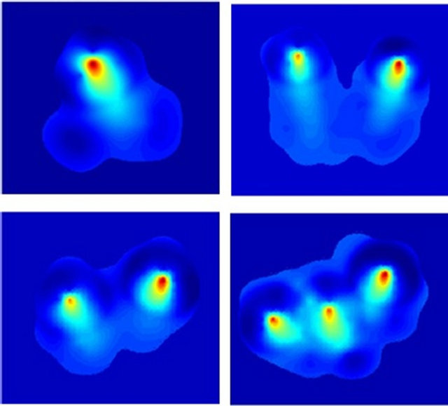
Figure 4. The concentration contour profile in different contaminant aquifers [76].
Therefore coupled and iterative sequential source identification and dynamic monitoring network design framework is required. The coupled approach provides a framework for necessary sequential exchange of information between monitoring network and source identification methodology.
A schematic diagram of sequential identification of sources and design of monitoring network is shown in Figure 5. The preliminary identification of unknown sources, based on limited concentration data from existing arbitrary located wells, provides the initial rough estimation of the source fluxes. These identified source fluxes are then utilized for designing an optimal monitoring network for the first stage. The contaminant concentration data collected from the new designed monitoring network are utilized, as feedback information, to identify the source characteristics. Both the monitoring network and source identification process are repeated until satisfactory source characteristics are achieved.
Mahar and Datta [52] presented a methodology combining an optimal ground-water quality monitoring network design and an optimal source identification model. In the first step, using nonlinear optimization model embedding the flow and transport simulation models as constraints, preliminary identification of sources based on arbitrary located monitoring network was done.
In the next step, an integer programming formulation with the objective function minimizing the sum of concentrations for each time period at all potential monitoring points where a monitoring well has not be installed, selected the monitoring wells in subsequent time periods. In the last step, simulated concentrations at new monitoring wells were also perturbed to show the measurement
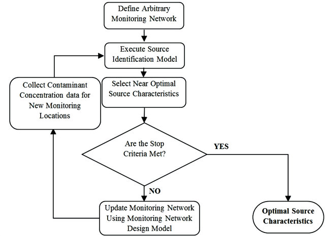
Figure 5. Schematic representations of the integrated source identification and monitoring network design models.
errors. To consider the model and parameter uncertainty, the source fluxes were perturbed by adding a random error with uniform distribution. Ten perturbations of source fluxes were generated and then the solute transport simulation model was solved for each perturbed set of fluxes to generate 10 different contamination plumes. The designed monitoring well locations were utilized for more accurate identification of source characteristics. Comparison of solution results shows that where there is no uncertainty in parameter or measurements, using data collected from an existing arbitrary monitoring network for source identification results in acceptable estimation of source fluxes, although properly designed monitoring network is preferable. In the presence of various uncertainties, existing monitoring network is not adequate and update or redesign is required.
Datta et al. [77] proposed a methodology which is an improvement over the combined source identification and monitoring network design model presented by Mahar and Datta [52]. Contrary to Mahar and Datta [52] using all perturbed plume realization for monitoring network design, they used the trimmed mean concentration incorporated in the monitoring network design. Using this method, the effect of extreme concentrations resulting from randomly generated fluxes can be minimized. These unacceptable or outlier concentrations at a potential monitoring network well location may be generated due to randomly generated source fluxes lying in the tail regions of distribution. They demonstrated the potential applicability of the developed methodology for an illustrative area.
Dokou and Pinder [78] addressed the issue of identifying and delineating of Dense Non-aqueous Phase Liquids (DNAPLs) at its sources. They proposed search strategy employs a series of mathematical tools, to provide optimal water quality sampling locations that reduce the uncertainty in the modelled concentration field. At the same time, the source locations are delineated with more certainty. In this research the iterative process of source identification and monitoring network design was proposed aimed to combine water quality information (hard data) with expert knowledge (soft data) into the integrated method. They assumed the hydraulic conductivity as an uncertain model parameter where other hydrogeological parameters were assumed to be deterministic. The iterative proposed search algorithm contains following steps.
1) Based upon available field information, approximate source locations were assumed. Using fuzzy membership functions, membership degree was assigned to each source location candidate considering how near they are to critical contaminant pollutants in domain. The Choquet integral, integrated the distance membership values and possibility of occurrence (assigned by expert judgment) for each candidate source.
2) To model the uncertainty in model parameter, different realizations of hydraulic conductivity field were generated. The Monte Carlo probabilistic and Latin Hyper Cube sampling techniques were utilized.
3) To calculate the concentration plume statistics, Monte-Carlo technique was utilized. The concentration results for each realization and each nodal location were used to calculate the concentration mean (called composite plume) and variencecovarience matrix.
4) Two factors were taken into account when deciding where to collect concentration sample: the reduction in the overall uncertainty resulting from taking a sample at a particular location (calculated using Kalman filter) and the distance of the sampling point from the source location). These two important features were combined using Choqute integral to produce a score for each potential sampling location. The location with the largest score was selected as the optimal sampling point.
5) After a sample was taken at the optimal point, the Kalman filter was used again to update the concentration mean and variance-covariance matrix with the real data.
6) Each individual plume was compared to the updated composite plume using a method that involves the use of fuzzy sets and their α-cuts. This strategy found the degree of similarity between the plumes by calculating a measure of common area between them. This degree of similarity was normalized and a new set of weight was assigned to each potential source location.
7) This new weights were used to calculate the new composite plume and repeating steps 3 to 6. The process was repeated until convergence on an optimal source location was achieved.
In this research the linear programming optimization method using response matrix simulation model selected the set of optimal source strengths. A two-dimensional homogenous hypothetical aquifer was studied to show the capability of proposed methodology. The results of sensitivity analysis concluded that the most important parameters include the type of α-cuts, used at the plume comparison step, and the pair of weights of importance, involved in the Choquet integral, used for the selection of the optimal water quality sampling location. The threedimensional extension and field application of this method were tested by Dokou and Pinder [79].
Singh and Datta [80] proposed a Kriging linked SA model for the spatial and temporal estimation of contaminant plume. The sequential simulation optimization model design the optimal monitoring network based on the objective function of minimizing the contaminant mass estimation error. The new selected monitoring wells generate feedback information for the SA optimization model to estimate the pollutant concentration plume more accurately.
6. Identification of Distributed Sources Characteristics
In most of the reported researches, the point sources were considered. However, the distributed or non-point sources will also produce widespread and long-lasting contamination in groundwater. Some common distributed sources of contamination are as follow;
• Contamination from agricultural chemical usage.
• Contamination carried by recharge from rain or snow water in to the ground.
• Contamination from large scale overland or underground waste dumps.
Figure 6 shows an abounded mine site. The mining waste dums, tailing ponds and lakes formed from flooding of the open-cuts, are different distributed sources of contamination in this area. The contamination in these sites adversely affects the quality of surface water and groundwater in the area. The leakage from the distributed sites may affect all the groundwater resources in neighborhood area and changed them to unusable water. Therefore selecting of appropriate remediation strategy is necessary.
The effectiveness of any remediation of contaminant groundwater is highly dependent on accurate characterization of the contaminant sources. Information about the location and the start time of activation of distributed sources are mostly available. The source identification model should be able to estimate the contaminant fluxes released from distributed sources as a function of time.
7. Future Directions and Conclusions
Selection of appropriate remediation strategy for management and control of aquifer contamination requires accurate and reliable source identification. Characterization of unknown pollutant sources remains a challenging problem due to the complex nature of real-life contaminated aquifers.
There are still areas which need further attention to increase the efficiency and applicability of source identifycation models in real contaminated areas.
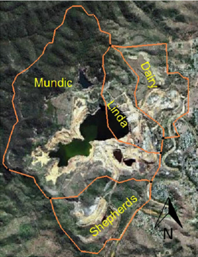
Figure 6. Distributed sources of contamination in an abandoned mine site [81].
In most of the study areas, the information available about geographic and hydro-geologic parameter values is sparse and inaccurate. The source identification model uses the simulation model to predict the contaminant concentration at monitoring locations, corresponding to each candidate source characteristics. The un-modelled uncertainty due to the presence of uncertainty about geographic and hydro-geologic parameter values, reduce the accuracy of source identification model. Further methods should be utilized to consider this un-modelled uncertainty more systematically. Fuzzy logic is one of the methods which can be incorporated to model parameter uncertainty in source identification procedure. The authors of this article are already engaged in extending source identification methodologies to incorporate fuzzy logic.
The feedback based iterative and sequential procedure of monitoring network design and source identification can effectively increase the efficiency of both models. Further studies considering real-life contaminant aquifers are required to refine such integrated methodologies. In recent years, a large number of contaminant aquifer sites have been identified for remediation in which the sources of contamination are distributed ones. The application of source identification and monitoring network design models needs to be expanded to incorporate overland and underground distributed sources, such as those present in mining sites now abandoned after extraction.
Many of the simulation models described in literature considered the transport of contamination result of advection and dispersion. The reaction procedures dominate the transport process of many contaminants. The geo-chemistry of contaminants needs to be considered and adequately modelled in source identification and monitoring network design models. Incorporating the reaction terms in transport simulation model, increase the complexity of model. The temperature, humidity, and pH are some of the parameters which need to be considered by including the reaction term in simulation model. The development of a versatile and meaningful methodology for accurate and reliable characterization of groundwater pollution sources has become a reality, even in the presence of usual parameter, modelling and measurement uncertainties. An integrated approach of optimal source identification and feedback of information from a sequentially designed monitoring network have enhanced the capability for designing effective remediation strategies for sustainable use of groundwater aquifers.
8. Acknowledgements
The work has been supported by the CRC for Contamination Assessment and Remediation of Environment, Australia.
REFERENCES
- S. S. D. Foster and P. J. Chilton, “Groundwater: The Processes and Global Significance of Aquifer Degradation,” Philosophical Transactions of the Royal Society of London. Series B: Biological Sciences, Vol. 358, No. 1440, 2003, pp. 1957-1972. doi:10.1098/rstb.2003.1380
- S. Chadalavada, B. Datta and R. Naidu, “Optimal Identification of Groundwater Pollution Sources Using Feedback Monitoring Information: A Case Study,” Environmental Forensics, Vol. 13, No. 2, 2012, pp. 140-153. doi:10.1080/15275922.2012.676147
- A. N. Tikhonov and V. Y. Arsenin, “Solutions of IllPosed Problems,” American Mathematical Society, Providence, 1978.
- K. Schulz and B. Huwe, “Water Flow Modeling in the Unsaturated Zone with Imprecise Parameters using a Fuzzy Approach,” Journal of Hydrology, Vol. 201, No. 1-4, 1997, pp. 211-229. doi:10.1016/S0022-1694(97)00038-3
- N.-Z. Sun, “Inverse Problems in Groundwater Modeling,” Klumer Academic Publisher, Boston, 1994.
- L. W. Gelhar, “Stochastic Subsurface Hydrology from Theory to Applications,” Water Resources Research, Vol. 22, No. 9S, 1986, p. 135. doi:10.1029/WR022i09Sp0135S
- A. C. Bagtzoglou, A. F. B. Tompson and D. E. Dougherty, “Probabilistic Simulation for Reliable Solute Source Identification in Heterogeneous Porous Media,” NATO ASI Series, Water Resources Engineering Risk Assessment, 1991.
- A. C. Bagtzoglou, A. F. B. Tompson and D. E. Dougherty, “Application of Particle Methods to Reliable Identification of Groundwater Pollution Sources,” Water Resources Management, Vol. 6, 1, 1992, pp. 15-23. doi:10.1007/BF00872184
- T. H. Skaggs and Z. J. Kabala, “Recovering the Release History of a groundwater Contaminant Plume—Method of Quasi-Reversibility,” Water Resources Research, Vol. 31, No. 11, 1995, pp. 2669-2673. doi:10.1029/95WR02383
- A. D. Woodbury and T. J. Ulrych, “Minimum Relative Entropy Inversion: Theory and Application to Recovering the Release History of a Groundwater Contaminant,” Water Resources Research, Vol. 32, No. 9, 1996, pp. 2671- 2681. doi:10.1029/95WR03818
- M. F. Snodgrass and P. K. Kitanidis, “A Geostatistical Approach to Contaminant Source Identification,” Water Resources Research, Vol. 33, No. 4, 1997, pp. 537-546. doi:10.1029/96WR03753
- M. M. Aral, “Aquifer Parameter Prediction in Leaky Aquifers,” Journal of Hydrology, Vol. 80, No. 1-2, 1985, pp. 19-44. doi:10.1016/0022-1694(85)90073-3
- G. K. Mahinthakumar and M. Sayeed, “Hybrid Genetic Algorithm—Local Search Methods for Solving Groundwater Source Identification Inverse Problems,” Water Resources Planning and Management, Vol. 131, No. 1, 2005, pp. 45-57. doi:10.1061/(ASCE)0733-9496(2005)131:1(45)
- J. Atmadja and A. C. Bagtzoglou, “State of the Art Report on Mathematical Methods for Groundwater Pollution Source Identification,” Environmental Forensics, Vol. 2, No. 3, 2001, pp. 205-205. doi:10.1006/enfo.2001.0055
- B. J. Wagner, “Simultaneous Parameter Estimation and Contaminant Source Characterization for Coupled Groundwater Flow and Contaminant Transport Modelling,” Journal of Hydrology, Vol. 135, No. 1, 1992, pp. 275-303. doi:10.1016/0022-1694(92)90092-A
- T. H. Skaggs and Z. J. Kabala, “Recovering the Release History of a Groundwater Contaminant,” Water Resources Research, Vol. 30, No. 1, 1994, pp. 71-79. doi:10.1029/93WR02656
- C. X. Liu and W. P. Ball, “Application of Inverse Methods to Contaminant Source Identification from Aquitard Diffusion Profiles at Dover AFB, Delaware,” Water Resources Research, Vol. 35, No. 7, 1999, pp. 1975-1985. doi:10.1029/1999WR900092
- T. H. Skaggs and Z. J. Kabala, “Limitations in Recovering the History of a Groundwater Contaminant Plume,” Journal of Contaminant Hydrology, Vol. 33, No. 3, 1998, pp. 347-359. doi:10.1016/S0169-7722(98)00078-3
- R. M. Neupauer, B. Borchers and J. L. Wilson, “Comparison of Inverse Methods for Reconstructing the Release History of a Groundwater Contamination Source,” Water Resources Research, Vol. 36, No. 9, 2000, pp. 2469-2475. doi:10.1029/2000WR900176
- S. M. Gorelick, B. Evans and I. Remson, “Identifying Sources of Groundwater Pollution: An Optimization Approach,” Water Resources Research, Vol. 19, No. 3, 1983, pp. 779. doi:10.1029/WR019i003p00779
- B. J. Wagner and S. M. Gorelick, “A Statistical Methodology for Estimating Transport Parameters: Theory and Applications to One-Dimensional Advective-Dispersive Systems,” Water Resources Research, Vol. 22, No. 8, 1986, p. 1303. doi:10.1029/WR022i008p01303
- B. Datta, J. E. Beegle, M. L. Kavvas and G. T. Orlob, “Development of an Expert System Embedding Pattern Recognition Techniques for Pollution Source Identification,” National Technical Infortmation Service, Springfield, 1989.
- P. S. Mahar and B. Datta, “Optimal Identification of GroundWater pollution Sources and Parameter Estimation,” Water Resources Planning and Management, Vol. 127, No. 1, 2001, pp. 20-29. doi:10.1061/(ASCE)0733-9496(2001)127:1(20)
- B. Datta, D. Chakrabarty and A. Dhar, “Identification of Unknown Groundwater Pollution Sources Using Classical Optimization with Linked Simulation,” Journal of Hydro-Environment Research, Vol. 5, No. 1, 2011, pp. 25- 36. doi:10.1016/j.jher.2010.08.004
- S. Chadalavada, B. Datta and R. Naidu, “Optimisation Approach for Pollution Source Identification in Groundwater: An Overview,” International Journal of Environment and Waste management, Vol. 8, No. 1-2, 2011, pp. 40-61. doi:10.1504/IJEWM.2011.040964
- M. M. Aral, J. Guan and M. L. Maslia, “Identification of Contaminant Source Location and Release History in Aquifers,” Journal of Hydrologic Engineering, Vol. 6, No. 3, 2001, pp. 225-234. doi:10.1061/(ASCE)1084-0699(2001)6:3(225)
- R. M. Singh and B. Datta, “Identification of Groundwater Pollution Sources using GA-Based Linked Simulation Optimization Model,” Journal of Hydrologic Engineering, Vol. 11, No. 2, 2006, pp. 101-109. doi:10.1061/(ASCE)1084-0699(2006)11:2(101)
- G. K. Mahinthakumar and M. Sayeed, “Reconstructing Groundwater Source Release Histories Using Hybrid Optimization Approaches,” Environmental Forensics, Vol. 7, No. 1, 2006, pp. 45-54. doi:10.1080/15275920500506774
- H.-D. Yeh, T.-H. Chang and Y.-C. Lin, “Groundwater Contaminant Source Identification by a Hybrid Heuristic Approach,” Water Resources Research, Vol. 43, No. 9, 2007, pp. 1-16. doi:10.1029/2005WR004731
- L. He, G. H. Huang and H. W. Lu, “A Coupled Simulation-Optimization Approach for Groundwater Remediation Design under Uncertainty: An Application to a Petroleum-Contaminated Site,” Environmental Pollution, Vol. 157, No. 8, 2009, pp. 2485-2492. doi:10.1016/j.envpol.2009.03.005
- B. Datta, D. Chakrabarty and A. Dhar, “Simultaneous Identification of Unknown Groundwater Pollution Sources and Estimation of Aquifer Parameters,” Journal of Hydrology, Vol. 376, No. 1-2, 2009, pp. 48-57. doi:10.1016/j.jhydrol.2009.07.014
- M. K. Jha and B. Datta, “Simulated Annealing Based Simulation-Optimization Approach for Identification of Unknown Contaminant Sources in Groundwater Aquifers,” Desalination and Water Treatment, Vol. 32, No. 1-3, 2011, pp. 79-85. doi:10.5004/dwt.2011.2681
- C. Zheng, M. C. Hill and P. A. Hsieh, “Modflow-2000, The US Geological Survey Modular Ground-Water ModelUser Guid to the LMT6 Package, The Linkage with MT3DMS for Multi-Species Mass Transport Modeling,” Open File Report 01-82, USG SURVEY Denver, Colorado, 2001.
- C. Zheng and P. P. Wang, “A Modular Three-Dimensional Multispecies Transport Model for Simulation of Advection, Dispersion, and Chemical Reactions of Contaminants in Groundwater Systems, Documentation and User’s Guide,” University of Alabama, Tuscaloosa, 1999.
- C. Zheng and P. P. Wang, “A Field Demonstration of the Simulation Optimization Approach for Remediation System Design,” Ground Water, Vol. 40, No. 3, 2002, pp. 258-266. doi:10.1111/j.1745-6584.2002.tb02653.x
- M. Jha and B. Datta, “Three Dimensional Groundwater Contamination Source Identification Using Adaptive Simulated Annealing,” Journal of Hydrologic Engineering, Vol. 18, No. 3, 2012, pp. 307-313. doi:10.1061/(ASCE)HE.1943-5584.0000624
- M. Jha and B. Datta, “Application of Simulated Annealing in Water Resources Management: Optional Solution of Groundwater Contamination Source Characterization Problem and Monitoring Network Design Problems,” In: M. De Sales Guerra Tsuzuki, Ed., Simulated Annealing Single and Multiple Objective Problems, InTech, Rijeka, 2012, pp. 157-174. doi:10.5772/45871
- R. M. Singh and B. Datta, “Groundwater Pollution Source Identification and Simultaneous Parameter Estimation Using Pattern Matching by Artificial Neural Network,” Environmental Forensics, Vol. 5, No. 3, 2004, pp. 143-153. doi:10.1080/15275920490495873
- R. M. Singh, B. Datta and A. Jain, “Identification of Unknown Groundwater Pollution Sources Using Artificial Neural Networks,” Water Resources Planning and Management, Vol. 130, No. 6, 2004, pp. 506-514. doi:10.1061/(ASCE)0733-9496(2004)130:6(506)
- R. M. Singh and B. Datta, “Artificial Neural Network Modeling for Identification of Unknown Pollution Sources in Groundwater with Partially Missing Concentration Observation Data,” Water Resources Management, Vol. 21, No. 3, 2007, pp. 557-572. doi:10.1007/s11269-006-9029-z
- H. A. Loaiciga, R. J. Charbeneau, L. G. Everett, G. E. Fogg, B. F. Hobbs and S. Rouhani, “Review of GroundWater Quality Monitoring Network Design,” Journal of Hydraulic Engineering, Vol. 118, No. 1, 1992, pp. 11-37. doi:10.1061/(ASCE)0733-9429(1992)118:1(11)
- ASCE Task Committee, “Long-Term Groundwater Monitoring Design; The State of The Art,” Reston, 2003.
- US EPA, “Roadmap to Long-Term Monitoring Optimization,” 2005.
- J. B. Kollat, P. M. Reed and R. M. Maxwell, “ManyObjective Groundwater Monitoring Network Design Using Bias-Aware Ensemble Kalman Filtering, Evolutionary Optimization, and Visual Analytics,” Water Resources Research, Vol. 47, No. 2, 2011, pp. 1-18. doi:10.1029/2010WR009194
- P. D. Meyer and E. D. Brill, Jr., “A Method for Locating Wells in a Groundwater Monitoring Network under Conditions of Uncertainty,” Water Resources Research, Vol. 24, No. 8, 1988, pp. 1277-1282. doi:10.1029/WR024i008p01277
- P. D. Meyer, A. J. Valocchi and J. W. Eheart, “Monitoring Network Design to Provide Initial Detection of Groundwater Contamination,” Water Resources Research, Vol. 30, No. 9, 1994, pp. 2647-2659. doi:10.1029/94WR00872
- N. B. Yenigül, A. M. M. Elfeki, J. C. Gehrels, C. V. D. Akker, A. T. Hensbergen and F. M. Dekking, “Reliability Assessment of Groundwater Monitoring Networks at Landfill Sites,” Journal of Hydrology, Vol. 308, No. 1, 2005, pp. 1-17. doi:10.1016/j.jhydrol.2004.10.017
- Y. Li and A. B. C. Hilton, “Optimal Groundwater Monitoring Design Using an Ant Colony Optimization Paradigm,” Environmental Modelling and Software, Vol. 22, No. 1, 2007, pp. 110-116. doi:10.1016/j.envsoft.2006.05.023
- S. E. Cieniawski, J. W. Eheart and S. Ranjithan, “Using Genetic Algorithms to Solve a Multiobjective Groundwater Monitoring Problem,” Water Resources Research, Vol. 31, No. 2, 1995, pp. 399-409. doi:10.1029/94WR02039
- B. Datta and S. D. Dhiman, “Chance-Constrained Optimal Monitoring Network Design for Pollutants in Ground Water,” Journal of Water Resources Planning and Management, Vol. 122, No. 3, 1996, pp. 180-188. doi:10.1061/(ASCE)0733-9496(1996)122:3(180)
- A. Dhar and B. Datta, “Multiobjective Design of Dynamic Monitoring Networks for Detection of Groundwater Pollution,” Water Resources Planning and Management, Vol. 133, No. 4, 2007, pp. 329-338. doi:10.1061/(ASCE)0733-9496(2007)133:4(329)
- P. S. Mahar and B. Datta, “Optimal Monitoring Network and Ground-Water-Pollution Source Identification,” Water Resources Planning and Management, Vol. 123, No. 4, 1997, pp. 199-207. doi:10.1061/(ASCE)0733-9496(1997)123:4(199)
- I. Bogardi, A. Bardossy and L. Duckstein, “Effect of Parameter Uncertainty on Calculated Sediment Yield,” Advances in Water Resources, Vol. 8, No. 2, 1985, pp. 96- 101. doi:10.1016/0309-1708(85)90006-5
- D. C. McKinney and D. P. Loucks, “Network Design for Predicting Groundwater Contamination,” Water Resources Research, Vol. 28, No. 1, 1992, pp. 133-147. doi:10.1029/91WR02397
- L. M. Nunes, E. Paralta, M. C. Cunha and L. Ribeiro, “Groundwater Nitrate Monitoring Network Optimization with Missing Data,” Water Resources Research, Vol. 40, No. 2, 2004, pp. 1-18. doi:10.1029/2003WR002469
- G. Passarella, M. Vurro, V. D'Agostino and M. J. Barcelona, “Cokriging Optimization of Monitoring Network Configuration Based on Fuzzy and Non-Fuzzy Variogram Evaluation,” Environmental Monitoring and Assessment, Vol. 82, No. 1, 2003, pp. 1-21. doi:10.1023/A:1021662705554
- W. Woldt, I. Bogardi, W. E. Kelly and A. Bardossy, “Evaluation of Uncertainty in a 3-Dimensional Groundwater Contamination Plume,” Journal of Contaminant Hydrology, Vol. 9, No. 3, 1992, pp. 271-288. doi:10.1016/0169-7722(92)90008-3
- H. A. Loaiciga, “An Optimization Approach for Groundwater Quality Monitoring Network Design,” Water Resources Research, Vol. 25, No. 8, 1989, pp. 1771-1782. doi:10.1029/WR025i008p01771
- J. B. Kollat and P. M. Reed, “A Framework for Visually Interactive Decision-Making and Design Using Evolutionary Multi-Objective Optimization (VIDEO),” Environmental Modelling and Software, Vol. 22, No. 12, 2007, pp. 1691-1704. doi:10.1016/j.envsoft.2007.02.001
- [61] P. Reed and B. S. Minsker, “Striking the Balance: LongTerm Groundwater Monitoring Design for Conflicting Objectives,” Water Resources Planning and Management, Vol. 130, No. 2, 2004, pp. 140-149. doi:10.1061/(ASCE)0733-9496(2004)130:2(140)
- [62] G. S. Herrera and G. F. Pinder, “Space-Time Optimization of Groundwater Quality Sampling Networks,” Water Resources Research, Vol. 41, No. 12, 2005, pp. 1-15. doi:10.1029/2004WR003626
- [63] Y. Zhang, G. F. Pinder and G. S. Herrera, “Least Cost Design of Groundwater Quality Monitoring Networks,” Water Resources Research, Vol. 41, No. 8, 2005, pp. 1- 12. doi:10.1029/2005WR003936
- [64] P. Reed, B. Minsker and A. J. Valocchi, “Cost-Effective Long-Term Groundwater Monitoring Design using a Genetic Algorithm and Global Mass Interpolation,” Water Resources Research, Vol. 36, No. 12, 2000, pp. 3731- 3741. doi:10.1029/2000WR900232
- [65] J. Wu, C. Zheng and C. C. Chien, “Cost-Effective Sampling Network Design for Contaminant Plume Monitoring under General Hydrogeological Conditions,” Journal of Contaminant Hydrology, Vol. 77, No. 1-2, 2005, pp. 41-65. doi:10.1016/j.jconhyd.2004.11.006
- [66] J. Wu, C. Zheng, C. C. Chien and L. Zheng, “A Comparative Study of Monte Carlo Simple Genetic Algorithm and Noisy Genetic Algorithm for Cost-Effective Sampling Network Design under Uncertainty,” Advances in Water Resources, Vol. 29, No. 6, 2006, pp. 899-911. doi:10.1016/j.advwatres.2005.08.005
- [67] H. J. Montas, R. H. Mohtar, A. E. Hassan and F. A. AlKhal, “Heuristic Space-Time Design of Monitoring Wells for Contaminant Plume Characterization in Stochastic Flow Fields,” Journal of Contaminant Hydrology, Vol. 43, No. 3-4, 2000, pp. 271-301. doi:10.1016/S0169-7722(99)00108-4
- [68] P. F. Hudak, “A Method for Designing Configurations of Nested Monitoring Wells near Landfills,” Hydrogeology Journal, Vol. 6, No. 3, 1998, pp. 341-348. doi:10.1007/s100400050157
- [69] P. F. Hudak, H. A. Loaiciga and M. A. Marino, “Regional-Scale Ground Water Quality Monitoring via Integer Programming,” Journal of Hydrology, Vol. 164, No. 1-4, 1995, pp. 153-170. doi:10.1016/0022-1694(94)02559-T
- [70] P. Mugunthan and C. A. Shoemaker, “Time Varying Optimization for Monitoring Multiple Contaminants under Uncertain Hydrogeology,” Bioremediation Journal, Vol. 8, No. 3-4, 2004, pp. 129-146. doi:10.1080/10889860490887509
- [71] P. F. Hudak, “Effective Contaminant Detection Networks in Uncertain Groundwater Flow Fields,” Waste Management, Vol. 21, No. 4, 2001, pp. 309-312. doi:10.1016/S0956-053X(00)00079-9
- [72] J. B. Kollat and P. M. Reed, “A Computational Scaling Analysis of Multiobjective Evolutionary Algorithms in Long-term Groundwater Monitoring Applications,” Advances in Water Resources, Vol. 30, No. 3, 2007, pp. 408-419. doi:10.1016/j.advwatres.2006.05.009
- [73] S. Chadalavada and B. Datta, “Dynamic Optimal Monitoring Network Design for Transient Transport of Pollutants in Groundwater Aquifers,” Water Resources Management, Vol. 22, No. 6, 2008, pp. 651-670. doi:10.1007/s11269-007-9184-x
- [74] A. Dhar and B. Datta, “Global Optimal Design of Ground Water Monitoring Network Using Embedded Kriging,” Ground Water, Vol. 47, No. 9, 2009, pp. 806-815. doi:10.1111/j.1745-6584.2009.00591.x
- [75] A. Dhar and B. Datta, “Logic-Based Design of Groundwater Monitoring Network for Redundancy Reduction,” Water Resources Planning and Management, Vol. 136, No. 1, 2010, pp. 88-93. doi:10.1061/(ASCE)0733-9496(2010)136:1(88)
- [76] S. Chadalavada, B. Datta and R. Naidu, “Uncertainty Based Optimal Monitoring Network Design for a Chlorinated Hydrocarbon Contaminated Site,” Environmental Monitoring and Assessment, Vol. 173, No. 1-4, 2011, pp. 929-940. doi:10.1007/s10661-010-1435-2
- [77] O. Prakash and B. Datta, “Sequential Optimal Monitoring Network Design and Iterative Spatial Estimation of Pollutant Concentration for Identification of Unknown Groundwater Pollution Source Locations,” Environmental Monitoring and Assessment, 2012, pp. 1-16. doi:10.1007/s10661-012-2971-8
- [78] B. Datta, D. Chakrabarty and A. Dhar, “Optimal Dynamic Monitoring Network Design and Identification of Unknown Groundwater Pollution Sources,” Water Resources Management, Vol. 23, No. 10, 2008, pp. 2031- 2049. doi:10.1007/s11269-008-9368-z
- [79] Z. Dokou and G. F. Pinder, “Optimal Search Strategy for the Definition of a DNAPL Source,” Journal of Hydrology, Vol. 376, No. 3, 2009, pp. 542-556. doi:10.1016/j.jhydrol.2009.07.062
- [80] Z. Dokou and G. F. Pinder, “Extension and Field Application of an Integrated DNAPL Source Identification Algorithm that Utilizes Stochastic Modeling and a Kalman Filter,” Journal of Hydrology, Vol. 398, No. 3, 2011, pp. 277-291. doi:10.1016/j.jhydrol.2010.12.029
- [81] D. Singh and B. Datta, “Sequential Characterization of Contaminant Plumes Using Designed Monitoring Network,” IAHR-APD Congress, 7th IUMWC, Auchland, 2010.
- [82] M. K. Jha and B. Datta, “Application of Unknown Groundwater Pollution Source Release History Estimation Methodology to Distributed Sources Incorporating Surface-Groundwater Interactions,” Journal of Hydrologic Engineering, 2013 (unpublished).