Energy and Power Engineering
Vol. 4 No. 3 (2012) , Article ID: 19016 , 4 pages DOI:10.4236/epe.2012.43018
The Tidal Stream Power Curve: A Case Study
The Department of Geography the University of Hull, University of Hull, Hull, UK
Email: j.hardisty@hull.ac.uk
Received August 5, 2011; revised September 20, 2011; accepted October 10, 2011
Keywords: Tidal Stream Power; Harmonic Tidal Time Series; Resource Analysis
ABSTRACT
It is important to understand the relationship between the ambient ebb and flood currents and the electricity generated by tidal stream power generators to minimise investment risk and to optimise power generation for distribution purposes. Such analyses no longer rely on average descriptions of the flow field or on single values for the device efficiency. In the present paper, we demonstrate a new method involving the integration of synthesised long termflow vectors with logistic descriptions of the device power curves. New experiments are then described with the Neptune Proteus vertical axis tidal stream power generator involving tow tests at speeds to 1.5 m·s–1 in William Wright Dock on the Humber. The results are used to derive appropriate coefficients in the logisticcurve and to estimate the device’s annual electrical output.
1. Introduction
As the pace of development in tidal stream power generators is accelerating, there are increasing efforts to formulate accurate and localised resource analysis methodologies and yield models. In general, the determination of the power output from tidal stream turbines requiresfirstly that the fluid speed is known over long periods of time and secondly that the relationship between the speed and the electrical power output can be determined. However, the flow experienced by tidal stream power devices is complex. Tidal streams accelerate, decelerate and reverse over varying depths in each tidal cycle and are, therefore, turbulent [1,2], unsteady and non-uniform and can exhibit conditions which vary from sub-critical through critical to supra-critical in each tidal cycle.
In general, resource analyses in the United Kingdom have focussed upon the estimation of the local, total or regional power. The UK Atlas of Offshore Renewable Energy Resources [3] provides an overview of the wind, wave and tidal potential in UK waters. The tidal resource was derived from the Proudman Oceanographic Laboratory’s High Resolution Continental Shelf numerical model at a resolution of one nautical mile (approximately 1.8 km).
Following the publication of the Atlas, two methodologies were developed to assess the total national or regional resource. Firstly, in the so called “farm methodology” it was assumed that that the extractable energy was effectively limitless and that the power generated would be a function of the number of turbines installed [4,5]. Alternatively, in the so called “flux methodology” it was assumed that the extractable energy is a known factor of the total energy flowing across a given section of the seabed. This fraction was called the Significant Impact Factor (SIF) and was tentatively set at 20% [6,7]. The flux method was used in the UK Tidal Stream Energy Resource Assessment [8,9] which concluded that the total extractable UK resource is about 18 TWh/y. The farm methodology was applied to 36 sites in UK waters [10] and assumed a device cut in velocity of 1 m·s–1, 45% efficiency and a rated velocity at 70% of the Mean Spring Current Peak speed to calculate that 3 GW of wave and tidal power generators could be installed by 2020.
The three stages Path to Power study [11-13] considered constraints on development and concluded that the long term tidal stream power potential would be around 3% - 5% of UK demand and that financing, grid access, permitting and planning were the main obstacles to development. The potential for Welsh [14] and Scottish [15] marine power have also been reviewed.
The harmonic approach [16] which is used here is analogous to the resource analysis methodology utilised for wind turbines and involves applying a suitable power transfer function to a long-term time series of the flow. Unlike wind, however, the tidal current speed vector is deterministic and is based, essentially, upon gravitational theory, whereas the windspeed is inherently probabilistic. Unlike wind, therefore, tidal stream power is both continuous and predictable. There are three stages in this methodology:
1) Determination of a long term (e.g. annual) time series of the tidal currents flow speed.
2) Determination of a power curve or transfer function.
3) The application of the power function to the time series to determine the device yield.
2. Flow Time Series
There are a number of techniques used to determine the flow speed, U(t), at the site including the deployment of instrumentation and the erection, calibration and implementation of a numerical flow model. The harmonic methodology [16,17] utilises the tidal species:
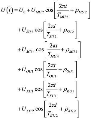 (1)
(1)
where UMU2, USU2, UMU4, UKU2, UKU1 and UOU1 are the amplitudes of the lunar semi-diurnal, solar semi-diurnal, lunar quarter diurnal, luni-solar semi-diurnal, luni-solar diurnal and lunar diurnal current velocities. TMU2 etc. are the corresponding periods taken as 12.4206, 12.0000, 6.2103, 11.9670, 23.93 and 25.82 hours and TMU2 etc. are the corresponding phase differences. Equation (1) was utilised to create a year-long, synthetic time series of the tidal flow at Hull Roads in The Humber Estuary within a software model entitled STEM (the Standard Tidal Energy Model, Hardisty, 2009) with harmonic amplitudes taken from British Admiralty data of UMU2 = 2.73, USU2 = 0.38. The results are shown in Figure 1 and incorporated into the yield assessment below.
3. Logistic Power Curves and Energy Yield
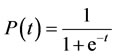
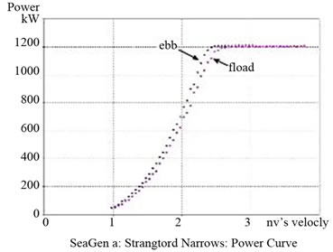
In many of the studies cited above [6,7,11,12] the device efficiency (the ratio of the electrical output power to the free stream hydraulic power over the capture area of the device) was usually included as a single number. More recently, however, power curves, which detail the relationship between power output and the tidal stream speed, have been developed. The power curve, as shown for example with Marine Current Turbine’s (MCT) data in Figure 2(a), is sigmoidal and rises from a threshold to an asymptotic maximum. For the present purposes, we examine the adoption of logistic function which is a common sigmoid curve often studied in relation to population growth [18]. The initial stage of growth is approximately exponential; then, as saturation begins, the growth slows and at maturity growth stops. A simple logistic function for the population as a function of time is defined by:
 (2)
(2)
The generalized logisticfunction is also known as the Richards’ curve which can be written in the present context as:
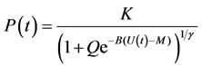 (3)
(3)
where P(t) is the instantaneous power output and the symbols are defined in Table 1 and fitted to the MCTdata as shown in Figure 2(a).
The annual energy yield, E W, for a tidal stream power generator is then summation, over the 8772 hours in an average year, of the application, usually at hourly intervals, of the logistic power curve derived to the varying values of the tidal stream flow derived in Section 2 above:
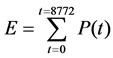 (4)
(4)
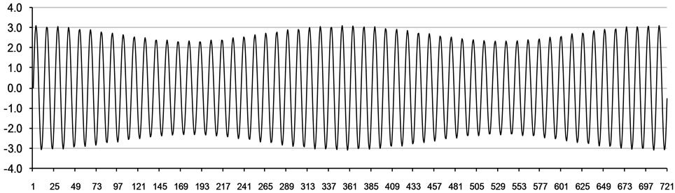
Figure 1. Example of 720 hr synthetic simulation of the tidal current speed, U(t) m·s–1 with flood positive at the Hull Roads Humber site.
 (a)
(a)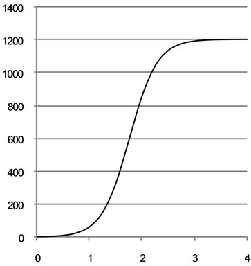 (b)
(b)
Figure 2. (a) Marine current turbines SeaGen power curve from http://www.marineturbines.com/3/news/article/38/dnv_confirms_seagen_s_powerful_performance_/; (b) Corresponding power curve simulated with the logistic function (Equation (3)) and the coefficient values shown in Table 1.
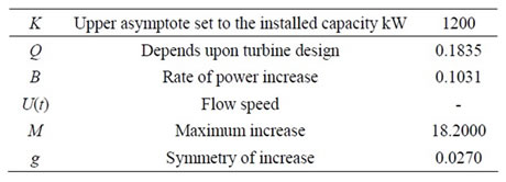
Table 1. Logistic coefficients and the corresponding values for the MCT device.
4. Experimental Data
The data were collected during test runs of the full scale, cross flow tidal stream power generator known as the Neptune Proteus NP1000 in order to provide support for the power curve and yield estimates for investment to cover device installation. The power generator is a floating structure designed to convert the kinetic energy of the flooding and ebbing of the tides into grid synchronised high voltage electricity. After modelling a wide range of approaches, Neptune identified the concept of a near shore, estuarine, vertical axis floating device to provide the maximum economic return on invested capital.
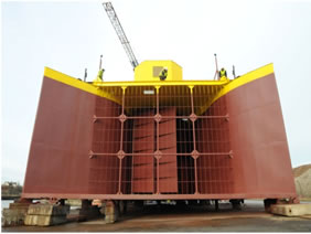
The 6 m × 6 m vertical axis turbine is housed within a Venturi duct (Figure 3) which accelerates the flow. The flow impact on the turbine is optimised by two computer controlled shutters and turbine torque feeds through a 1:200 Renold’s gearbox to a Brook Crompton, field current controlled, DC generator. Output from the device is fed through a Sprint microprocessor thyristor drive and 11 kV transformer to shore. The electronic and SCADA systems are shore mounted. Overall dimensions are 20.0 m × 12.8 m × 6.5 m (L × W × D).
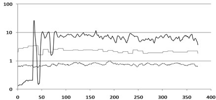
A series of dock tow trial experiments were conducted and results from two runs on 13th October 2010 are detailed here. In the first run, which commenced at 1208 GMT (Figure 4(a)), a range of parameters were measured including the vessel speed taken from an onboard GPS system and the output voltage and current which were used to calculate the electrical power generated. A second run which commenced at 1308 GMT (Figure 4(b)) was also analysed win detail and utilised the same logging equipment.
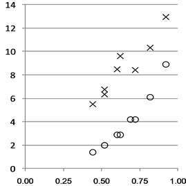
The results, as 1 Hz time series of speed, turbine RPM and electrical output for runs 1208 and 1308 are shown in Figures 4(a) and (b) respectively. Data sets were sampled from Runs 1208 and 1308 for a range of flow speeds over 30 s and 60 s intervals and the mean, maximum, minimum and standard deviation of each data set was determined. These parameters are plotted as X symbols in Figure 5(a) and are compared with the logistic power curve described earlier but with an upper asymptote plotted as O symbols. Whilst it is clear that the observations are in all cases above the corresponding power curve, a couple of riders must be borne in mind. Firstly, the dock trial data were enhanced by propeller wash from the towing tug, although the tug was more than 40 m in front of the device. Secondly, the production device performance will undoubtedly be enhanced by enechelon mooring arrangement and by the detailed CFD design of the duct, shutters and turbine.
The logistics power curve approach thus provides a reasonable estimate of the tidal stream power device’s behaviour and can then be used to derive additional design parameters as shown in Table 2.
Finally, the logistic power curve (Equation (3)) with the parameters in Table 1 and an upper asymptote of 250 kW was applied to the synthesised annual time series of flows at the Hull Roads Humber site derived from Equation (3) the estimate the annual yield in accordance with Equation (4). The result indicates an annual yield of about 1050 MWhr for the prototype device.
 (a)
(a)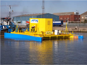 (b)
(b)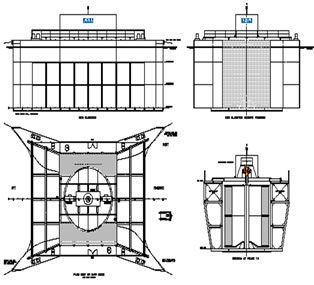 (c)
(c)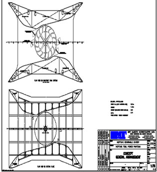 (d)
(d)
Figure 3. (a) Venturi duct entrance showing protection grid, shutters and turbine; (b) Generating electricity during tow tests at 1 m·s–1; (c) General arrangement showing for-aft sections and plan; (d) General arrangement showing 16 blade turbine and shutters.
 (a)
(a)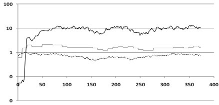 (b)
(b)
Figure 4. Time series of flow speed (lower line, broken, m·s–1), RPM (middle line, faint) and electrical power (upper line, solid, kW) for (a) Run 1208; (b) Run 1308 with generator excitation at 50%.
 (a)
(a) (b)
(b)
Figure 5. (a) Flow speed and power output for various subsamples of Run 1308and the comparison of the observed(X) and theoretical (O) results for power output kW versus the flow speed, m·s–1; (b) Data plotted on the “commercial” power curve for the Neptune NP1000.
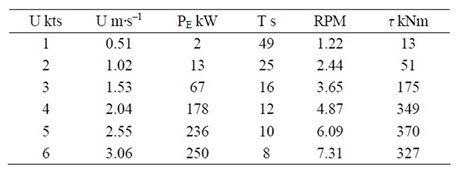
Table 2. Power characteristics for the Neptune Proteus demonstrator.
5. Conclusions
This paper has reviewed important works on the assessment of national, regional and local or turbine specific tidal stream power resources and device output. It has presented the harmonic method for the determination of long-term tidal stream vector time series. It has then developed the logistic equation to represent device power curves, and parameterised the equation with empirical data.
A case study is then presented in which the annual electrical energy output from the new Neptune Proteus NP1000 device was determined. The flow time series was determined from the application of the harmonic method to an estuarine site in Hull Roads on the Humber using British Admiralty amplitude, period and phase coefficients. The power curve was determined from the logistic equation using new data from dock tow trials of the device. The annual electrical power output was then calculated to be 1050 MWhr from the summation of the application of the power curve to hourly values of the flow.
REFERENCES
- K. F. Bowden and L. A. Fairbairn, “Measurements of Turbulent Fluctuations and Reynolds Stresses in a Tidal Current,” Proceedings of the Royal Society of London Series A, Vol. 237, No. 1210, 1956, pp. 422-438.
- Y. Lu, “Turbulence Characteristics in a Tidal Channel,” Journal of Physical Oceanography, Vol. 30, No. 5, 2000, pp. 855-867. doi:10.1175/1520-0485(2000)030<0855:TCIATC>2.0.CO;2
- ABPmer, “DTI Atlas of the Offshore Renewable Energy Resource,” Department of Trade and Industry, London, 2004.
- I. G. Bryden, T. Grinstead and G. T. Melville, “Assessing the potential of a Simple Tidal Channel to Deliver Useful Energy,” Applied Ocean Research, Vol. 26, No. 5, 2004, pp. 198-204. doi:10.1016/j.apor.2005.04.001
- C. Garrett and P. Cummins, “The Power Potential of Tidal Currents in channels,” Proceedings of the Royal Society of London Series A, Vol. 461, No. 2060, 2005, pp. 2563- 2572.
- A. Owen and I. G. Bryden, “A Novel Graphical Approach for Assessing Tidal Stream Energy Flux in the Channel Isles,” Journal of Marine Science and Environment, Vol. C4, 2006, pp. 49-55.
- I. G. Bryden, “Latest Tidal Research,” 2007. http://www.tidaltoday.com/tidal07/presentations/IanBryden.pdf
- Black and Veatch, “Tidal Stream Energy Resource and Technology Summary Marine Energy Challenge,” Carbon Trust, London, 2004.
- Black and Veatch, “Phase II UK Tidal Stream Energy Resource Assessment Marine Energy Challenge,” Carbon Trust, London, 2005.
- Environmental Change Institute, “Variability of UK Marine Resource,” Carbon Trust, London, 2005.
- ABPmer, “Path to Power Stage II: The Stakeholder/Statutory Bodies’ View on Development,” BWEA npower Juice, Edinburgh, 2006.
- Bond Pearce, “Path to Power Stage I: Wave and Tidal Energy around the UK Legal and Regulatory Requirements,” BWEA npower Juice, Edinburgh, 2006.
- Climate Change Capital, “The Path to Power,” BWEA npower Juice, Edinburgh, 2006.
- ABPmer, “Potential Nature Conservation and Landscape Impacts of Marine Renewable Energy Development in Welsh Territorial Waters,” Countryside Commission for Wales, Bangor, 2005.
- Faber Munsell and Metoc, “Scotish Marine Renewable Strategic Environmental Assessment Environmental Report,” Scottish Executive, Edinburgh, 2007.
- J. Hardisty, “The Analysis of Tidal Stream Power,” Wiley, Chichester, 2009.
- K. R. Dyer, “Estuaries: A Physical Introduction,” John Wiley & Sons Ltd., Chichester, 1997.
- F. J. Richards, “A Flexible Growth Function for empirical use,” Journal of Experimental Botany, Vol. 10, No. 2, 1959, pp. 290-300. doi:10.1093/jxb/10.2.290