Received 26 December 2014; revised 7 January 2015; accepted 22 January 2015

ABSTRACT

The study of the confluences of the roots of a given set of polynomials―root-pattern problem― does not appear to have been considered. We examine the situation, which leads us on to Young tableaux and tableaux representations. This in turn is found to be an aspect of multipartite partitions. We discover, and show, that partitions can be expressed algebraically and can be “differentiated” and “integrated”. We show a complete set of bipartite and tripartite partitions, indicating equivalences for the root-pattern problem, for select pairs and triples. Tables enumerating the number of bipartite and tripartite partitions, for small pairs and triples are given in an appendix.

Keywords:

Combinatorics, Partitions, Polynomials, Root-Patterns, Tableaux

1. Introduction

We are interested in the “root-patterns” or confluences of the roots of a given set of polynomials―a topic one may have expected would have been studied in depth in the 19th century. However, apart from results on Resultants etc., there does not appear to have been much further development.

Motivation for consideration here arises from General Relativity where the classification of the Lanczos-Zund (3,1) spinor involves various confluences of the roots of two cubics [1] . This in turn relates to the important aspect of Invariants of the spinor―much like the confluences of roots of a quartic form the various algebraic types for the Weyl spinor (Petrov classification) and are linked to its Invariants.

It is shown here how the root-patterns problem becomes a problem in partitions. In this context, from bipartite partitions, an application to derivations of spinor factorizations in General Relativity has been made [2] .

For example, given a quadratic and two cubics, a root-pattern may be indicated by ab, aad, bce where a, b are the roots of the quadratic and a, a, b and b, c, e are the roots of each of the cubics.

Three observations may be made. Firstly, the order of the polynomials is immaterial and so the root-pattern is also aad, ab, bce, or bce, aad, ab etc. Secondly, although we have written the roots of each polynomial in “ascending letter” order, the confluences of the roots or root-pattern is unchanged if we rearrange the letter order for each polynomial’s roots. Then the last root-pattern is also ebc, ada, ab. Thirdly, for any root-pattern, we can replace any letter by any other, unused, letter as the actual value of the root is unimportant. This then allows an interchange of letters, e.g., bce, aad, ab with the interchange becomes ace, bbd, ba. In other words, any permutation of letters is allowed.

From an initial set S, a collection of elements of S where elements can be repeated, and shown juxtaposed, is just a list. A list with r elements is an r-element list and is the degree of the corresponding polynomial whose roots are the elements of the list or tuple. We define a root-pattern as just a collection of lists. Thus, the root-pattern ab, aad, bce is the collection of lists ab and aad and bce where the initial set is. There are three elements in this root-pattern, a 2-element list or pair and two 3-element lists.

The number of lists in the collection is the number of polynomials. The number of components in a list is the degree of the polynomial.

If we take two polynomials, we refer to the binary case, for three polynomials, the ternary case etc.

The three observations we made earlier may now be formalized as the following rules.

1) Any two polynomials can be interchanged. This translates to any two lists in a root-pattern can be interchanged.

2) Any rearrangement of the ordering of roots of a polynomial translates as a rearrangement of the ordering of the roots in the corresponding list for that polynomial in the root-pattern.

3) Any permutation of the letters (roots) in the set of polynomials translates to a permutation of the letters in the root pattern.

It is the commonality or confluence of roots in the various polynomials that we are interested in.

We define two root-patterns A and B to be equivalent if B can be obtained from A by any of the three rules; otherwise they are inequivalent.

For the ternary case, the root patterns ab, aad, bce and bc, bvb, xcy are equivalent but neither are equivalent to aad, bb, acc.

For a given set of polynomials the various root-patterns, that is the combinations of the various roots, which include common roots, is of interest to us.

What we would like to obtain is the enumeration and the consequent collection of (inequivalent) root-patterns of several polynomials. More specifically, given m₁ linear forms, m₂ quadratics, ・・・, m_n n-ics, enumerate and determine the set of inequivalent root-patterns. This is the “root-pattern’ problem.

Let us first consider a simple example.

Two Quadratics

The roots of two quadratics (two lists of pairs,) are displayed in the form where the letters refer to the roots of the two polynomials. Besides using letters we also use corresponding numbers.

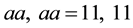all roots equal.

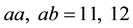roots of first are equal, which are common to one root of second.

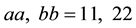roots of first are equal, but different to equal roots of second.

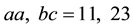roots of first are equal, but distinct to each root of second.

both distinct roots of first are duplicated in second.

roots of first and second have a common root, with each of the others distinct.

all roots of both quadratics are different.

There are 7 inequivalent cases which can be written as rows

Note, for example, that a case written as ab, cc (12, 33) is essentially the same as cc, ab (33, 12) since the order of the quadratics is immaterial. Then too cc, ab (33, 12) is also the same as case 4 aa, bc (11, 23), since the letters (and numbers) used do not matter.

2. Young Tableaux

It is seen that the roots of the two quadratics, displayed as rows, are instances of Young tableaux. We can always represent the roots of a set of polynomials as Young tableaux. For a polynomial of highest degree, say, we place its roots in a first or top row, and moving downwards to a second row with polynomials of the same or lesser degrees and so on, from top to bottom. The number of entries in row i is and is the length of the row. Thus for a tableaux of rows,. The root-patterns of any number of polynomials can be displayed as Young tableaux.

As the order of roots of a polynomial in any row is immaterial we will take it that the numbers in each row of a Young tableau are always arranged in weakly increasing order.

A question arises as to whether every tableau can be ordered so that every row and column is weakly increasing. This is in fact not so. For any permutation of and row interchanges, the tableau (with weakly increasing rows)

cannot be displayed as one with weakly increasing columns, also allowing for the interchange of any rows.

2.1. Tableau Representation

We will take it that the numbers used in any tableau of n rows will be consecutive, (the largest number in the tableau). Should any tableau contain q non-consecutive numbers we can always replace them so that we have consecutive numbering.

We now construct a different numbering on a tableau T. For a given T we form n-tuples or lists and there will be at most q of them. We will write the n-tuples or lists in sequence which we call the tableau representation. The entry of the tuple will be the number of times the number j appears in the row. Thus for the tableau T with rows and

count the number of times 1 appears in the first row of the tableau, next the number of times 1 appears in the second row and so on, written as 110, the first 3-tuple or list. Then count the number of times 2 appears in the first row, next the number of times 2 appears in the second row and so on, to get 002 etc., so that finally we construct the tableau representation 110, 002, 120, 100 of T.

From this representation, the tableau can be reconstructed as follows.

1) The sum of the first components of each triple tells us the length of the first row; similarly for the second and third. Thus for T we have a 3-rowed tableau with row lengths.

2) Since there are four triples there will be 4 different numbers 1, 2, 3, 4 used.

3) The first component of each 3-tuple tells us that the first row contains one 1, one 3 and one 4, so the first row is 134. Similarly the second row is 133 and the third row is 22. Putting these together, one row under another, in order, recovers T.

In the tableau representation of a set of polynomials, the tuple refers to the number j, the number in a tuple refers to the row of the tableau.

The 7 tableaux for two quadratics, namely

have the 7 tableaux representations

2.2. Nil-Addition and the Algebraic Representations of Partitions

Partitions may be represented in two ways: for example the partitions of the number (4) are: 4, 3 + 1, 2 + 2, 2 + 1 + 1, 1 + 1 + 1 + 1 and a second way as:. This latter notation is manifested by extracting, from the following products, the terms of degree 4

so that we have where the exponents are the partitions

which is the second notation.

The general rule for partitions of a single variable is given by a generating function [3] . Let be a set of positive intergers, usually. Then

where the exponent of is the partition This is seen in the above parttioning of the number (4).

For bipartite partitions the generating function for a set of pairs of positive integers, usually is

Expanding as a power series in and, the coefficient of is the number of bipartite partitions of. The process can be computerized and short tables of bipartite and tripartite partitions are displayed in the Appendix.

We will use the first notation, however, and consider bipartite partitions here.

The pair (2,1) has the following 4 (bi)partitions:

We have used a delimiting comma here, rather than the usual summation sign, since we will now use the summation sign to express the partitions as a “sum”

.

Any (bipartite) partition is a tuple/list of parts: thus, the partition 11, 10 has parts 11 and 10. Each part is comprised of components; the part 10 has components 1 and 0. Partitions are then shown as their tableau representations. Thus we can talk of a partition or a tableau representation of a tableau, and construct a tableau that represents the partition1.

The + symbol used here needs more definition. Whilst it will be legitimate to write there will be no point in writing since we are only interested in the single partition, not multiples of it. We avoid such “multiples” of partitions by adopting the rule for addition of a partition

We refer to the rule as the nil-addition of a partition.

The root-patterns of two quadratics, written (2,2) can then be shown as the sum of the 7 tableau representations, so that we now write

Note that the tableau representations and are equivalent respectively to and, the first by interchange of rows; the second, by interchanging the numbers 1 and 3 and then

interchanging rows. The root patterns are equivalent for these two. Including the latter two equivalent tableaux representations to the 7 above, we have

This is exactly the expression of the pair (2,2) into its 9 bipartite partitions.

The 7 tableau representations (or corresponding partitions) for the roots of two quadratics are a subset of the full set of tableau representations of all partitions of (2,2).

It is convenient to call the sum of all partitions of a given number, pair, triple etc., its partition representation.

Algebraic Representation

Parts and hence partitions of a number, pair of numbers etc., can be represented algebraically. For the bipartite case let x represent the tuple 10 and y the tuple 01. Then put, and etc. Such representations of parts or tableau representations we refer to as algebraic representations. The representation by monomials transfers partitions to algebraic notation obeying rules we have yet to set up

Let us denote the concatenation of two tuples by a concatenation (circle) symbol 2, as a concatenating operator, so that 20,01 is written and 10,10,01 is This notation will apply to all concatenation of tuples.

Besides the concatenation symbol, we introduce an extension symbol as an extension (or integrating) operator and develop some rules for “circle and extension multiplication”. Let be monomials.

We define the following laws

(1)

(2)

(3)

(4)

(5)

where ac etc., is the ordinary (dot・) multiplication of two monomials.

It is easily seen that, so that both and are commutative.

Rules (2), (3) and (4) allow us to simplify some of the calculations that are used, by employing simplified rules. Thus with in rule 4 we have

using nil-addition. Most often we will therefore use rule 4′

(4′)

Then with in 4′, we have which, also with nil-addition, gives a simple rule 5′ which we will very frequently employ

(5′)

The term is a monomial and the term is a concatenated term. It is clear that.

Rule 5 is a distributive law, and for simplified versions we have

Collating the rules that will be frequently used we have

(1)

(2)

(3)

(4′)

(5′)

(6′)

Note that (5′) is derivable from (4′) and that the rhs of consists of a monomial part and a concatenated part. It is also easily seen that

In these shortened versions of the original laws it may be convenient to use the terminology of an integating operator instead of that of the extension operator, using the symbol i rather than. With this notation we rewrite laws (4′), (5′) and (6′) as

(4′′)

(5′′)

(6′′)

Let, then rule (5′) gives. In terms of tuples where, y = 01 the monomial expression, where we see that the (dot) product or is the mere addition of the components 01 and 21.

The left table below shows an example of the use of the extension operator employed “algebraically”, with the rhs consisting of monomials, including concatenations of them. The right table shows the interpretation of these as tableau representations.

Example 1. Suppose we wish to obtain the tableau representation of (2,2) associated with the roots of two quadratics. It consists of the 9 partitions

We can construct the (2,2) partition representation from the algebraic representation of (2,1) The algebraic representation of is

To get the (2,2) algebraic representation from the (2,1) algebraic representation we multiply it by 01, that is by the monomial y, using the extension operator.

Taking each of the 4 terms separately we get, making simplifications and writing terms with preceding to reorder monomials in circle products,

Adding these up we have the algebraic representation of (2,2)

Ignoring the irrelevant numerical coefficients (nil-addition) in this 9 term algebraic representation of (2,2) we have

In terms of the partition representation this is

The actual tableau corresponding to each term in these expressions is easily constructed.

In the algebraic representation, the terms and are equivalent (interchange and), as also the terms and. The tableau representation is the equivalence of pairs 21, 01 and 12, 10 and pairs 20, 01, 01 and 10, 10, 02.

Thus we may consider the (2,2) partitioning as consisting of 7 inequivalent pairs. We may take this by defining an order (dominance) algebraically on the variables, say, x > y (thus ignoring the term) or (ignoring the latter term).

Alternatively we could “symmetrize” the expression and consider the set of symmetrised terms,

which are 7.

So really the problem of finding the number of inequivalent root-patterns of a set of polynomials (two quadratics here) is subsumed as that of determining the set of symmetrized partitions, a subset of all partitions corresponding to all tableau representations of the polynomials.

3. Differentiation of Partitions

Partitons now being expressed algebraically, provide an opportunity to introduce “differentiation”.

If a and b are monomials in x (they must be of the form and) we define a derivative operator such that

In practice we may just differentiate a monomial and ignore any coefficients. The derivative operator can be extended to a partial derivative operator such as in an obvious way etc.

Example 2. The tableau and algebraic partitioning of numbers (3) and (4) is

Ordinary differentiation of the latter (also using 2.) gives

which, ignoring coefficients, reduces to which is precisely the partitioning of (3).

The tableau and algebraic partitioning of the bivariate partitions (2,1) and (2,2) is

Differentiating the latter with respect to y gives

which all amounts to, ignoring coefficients,

precisely the partitioning of (2,1).

The process of differentiation in the example has exhibited the “downgrading” of partitions―from (4) to (3) and from (2,2) to (2,1). The reverse process of “integrating” or “upgrading” was performed in Example 1 in deriving the partitioning of (2,2) from (2,1).

4. Display of Partitioning for Low Degree Polynomials

The partition representations of low degree polynomials are displayed. Equivalent partitions are superscripted alike. The first-listed partition is the dominant one. Partitions of all different row lengths are necessarily all inequivalent. Partitions with equal row lengths will have partition equivalents. The algebraic representations can easily be constructed from the tableau representations.

4.1. Binary Root Patterns

4.1.1. Two Quadratics (2,2)

There are 9 possible partitions with 7 being inequivalent.

4.1.2. Cubic and Quadratic (3,2)

As the polynomials are of different degrees all partitions are inequivalent. There are 16 inequivalent partitions.

4.1.3. Two Cubics (3,3)

The total number of partitions is 31. The number of inequivalent ones (here) is 21.

Other partitions, equivalent to some listed here, are:

and, and etc.

4.2. Ternary Root-Patterns

4.2.1. A Cubic and Two Linear Forms (3,1,1)

The total number of partitions is 21. The number of inequivalent ones is 17.

It is easily seen that a partition is equivalent to a given partition if the and entries of each part of the partition are interchanged―corresponding to row interchanges in the tableau view of the partitions. More generally, any permutation of the numbers of a permutation gives an equivalent partition. Interchange of the parts of a partition produces an equivalent partition.

4.2.2. Two Quadratics and a Linear Form (2,2,1)

The total number of partitions is 26. The number of inequivalent ones is 20.

4.2.3. Three Quadratics (2,2,2)

The total number of partitions is 66. The number of inequivalent ones is 51.

References

Appendix

1. Bipartite Partitions

The table shows the number of bipartite partitions for for which is the coefficient of in a power series expansion of

2. Tripartite Partitions

The tables show the number of tripartite partitions for for which is the coefficient of in a power series expansion of

NOTES

¹Note that the partitions and tableau representations of the number (4) are: 4 = 1111; 3 + 1 = 1112; 2 + 2 = 1122; 2 + 1 + 1 = 1123; 1 + 1 + 1 + 1 = 1234.

²In fact the delimiting comma (,) denotes the concatenation but we use the circle symbol as it is mathematically more readable and a reminder that a new process is involved.

References

- Agacy, R.L. and Briggs, J.R. (1994) Algebraic Classification of the Lanczos Tensor by Means of Its (3,1) Spinor Equi- valent. Tensor, 55, 223-234.
- Agacy, R.L. (2002) Spinor Factorizations for Relativity. General Relativity and Gravitation, 34, 1617-1624. http://dx.doi.org/10.1023/A:1020116122418
- Andrews, G.E. (1984) The Theory of Partitions. Cambridge University Press, Cambridge. http://dx.doi.org/10.1017/CBO9780511608650