ABSTRACT

In [1], I. N. Vekua propose the Poincaré problem for some second order elliptic equations, but it can not be solved. In [2], the authors discussed the boundary value problem for nonlinear elliptic equations of second order in some bounded domains. In this article, the Poincaré boundary value problem for general nonlinear elliptic equations of second order in unbounded multiply connected domains have been completely investigated. We first provide the formulation of the above boundary value problem and corresponding modified well posed-ness. Next we obtain the representation theorem and a priori estimates of solutions for the modified problem. Finally by the above estimates of solutions and the Schauder fixed-point theorem, the solvability results of the above Poincaré problem for the nonlinear elliptic equations of second order can be obtained. The above problem possesses many applications in mechanics and physics and so on.

1. Formulation of the Poincaré Boundary Value Problem

Let D be an -connected domain including the infinite point with the boundary inwhere. Without loss of generality, we assume that D is a circular domain in, where the boundary consists of circles, and. In this article, the notations are as the same in References [1-8]. We consider the second order equation in the complex form

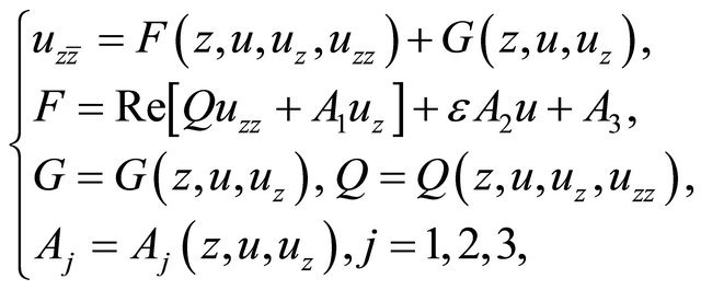(1.1)

satisfying the following conditions.

Condition C. 1), are continuous in for almost every point and for

2) The above functions are measurable in for all continuous functions in, and satisfy

(1.2)

in which are non-negative constants.

3) The Equation (1.1) satisfies the uniform ellipticity condition, namely for any number and w, U₁, the inequality

for almost every point holds, where is a non-negative constant.

4) For any function, , satisfies the condition

in which satisfy the condition

(1.3)

with a non-negative constant.

Now, we formulate the Poincaré boundary value problem as follows.

Problem P. In the domain D, find a solution of Equation (1.1), which is continuously differentiable in, and satisfies the boundary condition

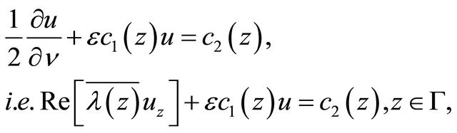(1.4)

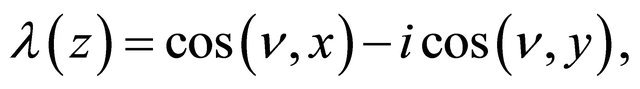
in which is any unit vector at every point on, and are known functions satisfying the conditions

(1.5)

where, , , are non-negative constants.

If and on, where n is the outward normal vector on, then Problem P is the Dirichlet boundary value problem (Problem D). If and on, then Problem P is the Neumann boundary value problem (Problem N), and if, and on, then Problem P is the regular oblique derivative problem, i.e. the third boundary value problem (Problem III or O). Now the directional derivative may be arbitrary, hence the boundary condition is very general.

The integer

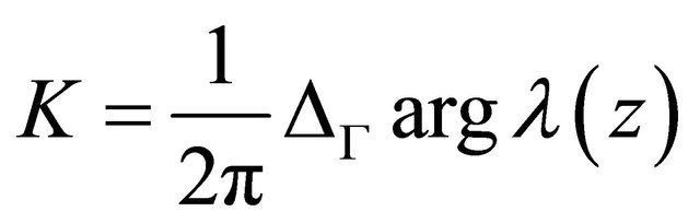
is called the index of Problem P. When the index Problem P may not be solvable, and when the solution of Problem P is not necessarily unique. Hence we consider the well-posedness of Problem P with modified boundary conditions.

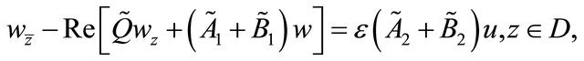
Problem Q. Find a continuous solution of the complex equation

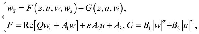(1.6)

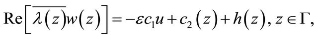
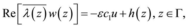
satisfying the boundary condition

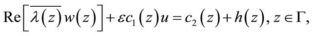(1.7)

and the relation

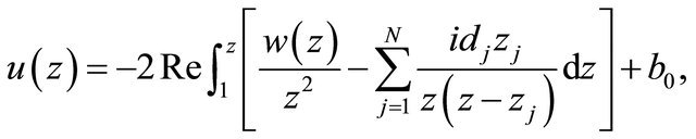(1.8)

where are appropriate real constants such that the function determined by the integral in (1.8) is single-valued in, and the undetermined function is as stated in

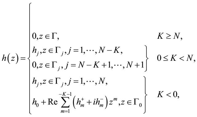
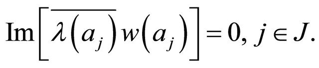
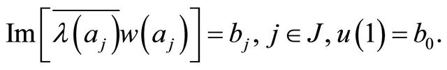
in which, are unknown real constants to be determined appropriately. In addition, for the solution is assumed to satisfy the point conditions

(1.9)

where

are distinct points, and are all real constants satisfying the conditions

(1.10)

for a non-negative constant.

2. Estimates of Solutions for the Poincaré Boundary Value Problem

First of all, we give a prior estimate of solutions of Problem Q for (1.6).

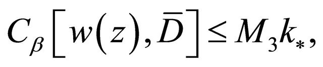
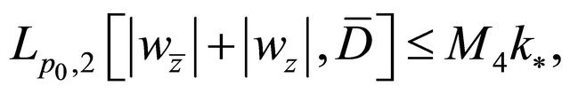
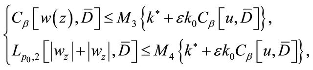
Theorem 2.1. Suppose that Condition C holds and ε = 0 in (1.6) and (1.7). Then any solution of Problem Q for (1.6) satisfies the estimates

(2.1)

(2.2)

in which

Proof. Noting that the solution of Problem Q satisfies the equation and boundary conditions

(2.3)

(2.4)

(2.5)

according to the method in the proof of Theorem 4.3, Chapter II, [2] or Theorem 2.2.1, [5], we can derive that the solution satisfies the estimates

(2.6)

(2.7)

where

and

From (1.8), it follows that

(2.8)

(2.9)

in which is a non-negative constant. Moreover, it is easy to see that

(2.10)

Combining (2.6)-(2.10), the estimates (2.1) and (2.2) are obtained.

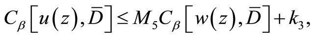
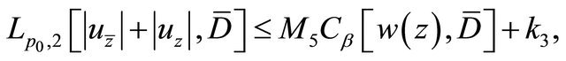
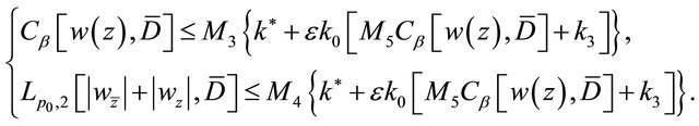
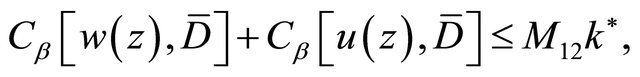
Theorem 2.2. Let the Equation (1.6) satisfy Condition C and in (1.6)-(1.7) be small enough. Then any solution of Problem Q for (1.6) satisfies the estimates

(2.11)

(2.12)

here are as stated in Theorem 2.1,

Proof. It is easy to see that satisfies the equation and boundary conditions

(2.13)

(2.14)

(2.15)

Moreover from (2.6) and (2.7), we have

(2.16)

and from (2.8)-(2.10), it follows that

(2.17)

If the positive constant is small enough such that, then the first inequality in (2.17) implies that

(2.18)

Combining (2.8) and (2.18), we obtain

(2.19)

which is the estimate (2.11). As for (2.12), it is easily derived from (2.9) and the second inequality in (2.17), i.e.

(2.20)

3. Solvability Results of the Poincaré Boundary Value Problem

We first prove a lemma.

Lemma 3.1. If satisfies the condition stated in Condition C, then the nonlinear mapping G:

defined by is continuous and bounded

(3.1)

where

Proof. In order to prove that the mapping:

Defined by is continuous, we choose any sequence of functions

such that

as Similarly to Lemma 2.2.1, [5], we can prove that

possesses the property

(3.2)

And the inequality (3.1) is obviously true.

Theorem 3.2. Let the complex Equation (1.1) satisfy Condition C, and the positive constant in (1.6) and (1.7) is small enough.

1) When, , Problem Q for (1.6) has a solution, where, , is a constant as stated before.

2) When Problem Q for (1.6) has a solution, where provided that

(3.3)

is sufficiently small.

3) If satisfy the conditions,  i.e. Condition C and for any functions

and, there are

(3.4)

where

is a sufficiently small positive constant, then the above solution of Problem Q is unique.

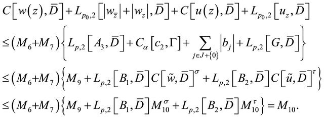
Proof. 1) In this case, the algebraic equation for t is as follows

(3.5)

where M₆, M₇ are constants as stated in (2.11) and (2.12). Because, , the Equation (3.5) has a unique solution Now we introduce a bounded, closed and convex subset B^* of the Banach space whose elements are of the form satisfying the condition

(3.6)

We choose a pair of functions and substitute it into the appropriate positions of

, in (1.6) and the boundary condition (1.7), and obtain

(3.7)

(3.8)

where

In accordance with the method in the proof of Theorem 1.2.5, [5], we can prove that the boundary value problem (3.7), (3.8) and (1.6) has a unique solution. Denote by the mapping from to. Noting that

provided that the positive number is sufficiently small, and noting that the coefficients of complex Equation (3.7) satisfy the same conditions as in Condition C, from Theorem 2.2, we can obtain

(3.9)

This shows that T maps B^* onto a compact subset in B^*. Next, we verify that T in B^* is a continuous operator. In fact, we arbitrarily select a sequence in B^*, such that

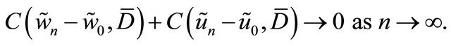(3.10)

By Lemma 3.1, we can see that

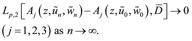(3.11)

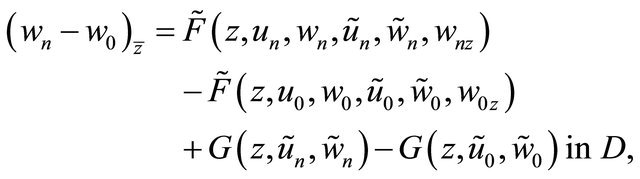
Moreover, from

,

it is clear that is a solution of Problem Q for the following equation

(3.12)

(3.13)

(3.14)

In accordance with the method in proof of Theorem 2.2, we can obtain the estimate

(3.15)

in which 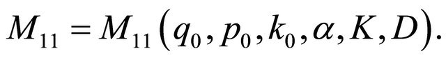From (3.10), (3.11) and the above estimate, we obtain

as

On the basis of the Schauder fixed-point theorem, there exists a function such that, and from Theorem 2.2, it is easy to see that, , and

is a solution of Problem Q for the Equation (1.6) and the relation (1.8) with the condition,.

In addition, if 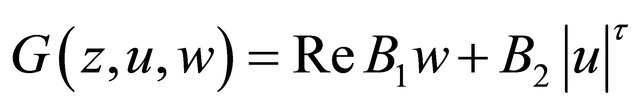inwhere then the above solvability result still hold by using the above similar method.

2) Secondly, we discuss the case: In this case, (3.5) has the solution provided that M₉ in (3.3) is small enough. Now we consider a closed and convex subset in the Banach space i.e.

(3.16)

Applying a method similar as before, we can verify that there exists a solution

of Problem Q for (1.6) with the condition

Moreover, if in D, where

, , j = 1, 2. Under the same condition, we can derive the above solvability result by the similar method.

3) When satisfies the condition (3.4), we can verify the uniqueness of solutions in this theorem. In fact, if, are two solutions of Problem Q for the Equation (1.6), then

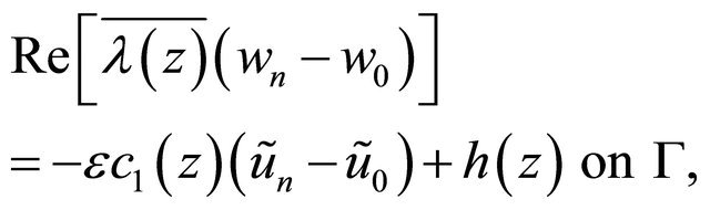
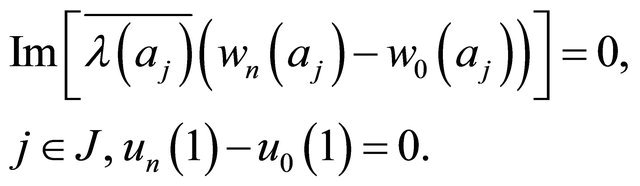
satisfies the equation and boundary conditions

(3.17)

(3.18)

(3.19)

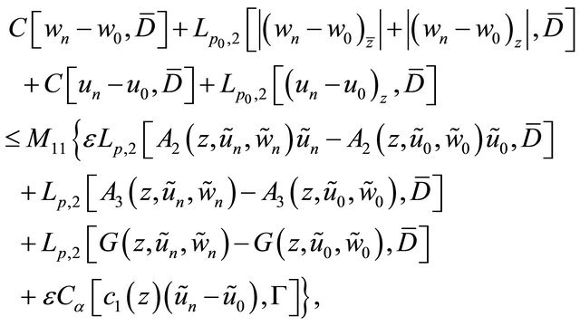
in which. Similarly to Theorem 2.2, we can derive the following estimates of the solution for complex Equation (3.17):

(3.20)

(3.21)

where

are two non-negative constants, Moreover the estimate

(3.22)

can be derived. Provided that the positive constant is small enough such that, from (3.22) it follows, i.e. in D. This completes the proof of the theorem.

From the above theorem, the next result can be derived.

Theorem 3.3. Under the same conditions as in Theorem 3.2, the following statements hold.

1) When the index K > N, Problem P for (1.1) has N solvability conditions, and the solution of Problem P depends on arbitrary real constants.

2) When Problem P for (1.1) is solvable, if solvability conditions are satisfied, and the solution of Problem P depends on arbitrary real constants.

3) When K < 0, Problem P for (1.1) is solvable under conditions, and the solution of Problem P depends on 1 arbitrary real constant.

Moreover, we can write down the solvability conditions of Problem P for all other cases.

Proof. Let the solution of Problem Q for (1.6) be substituted into the boundary condition (1.7) and the relation (1.8). If the function, i.e.

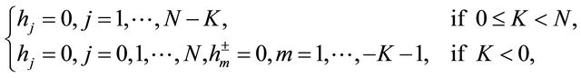
and, , then we have in D and the function is just a solution of Problem P for (1.1). Hence the total number of above equalities is just the number of solvability conditions as stated in this theorem. Also note that the real constants b₀ in (1.8) and in (1.9) are arbitrarily chosen. This shows that the general solution of Problem P for (1.1) includes the number of arbitrary real constants as stated in the theorem.

REFERENCES

- I. N. Vekua, “Generalized Analytic Functions,” Pergamon, Oxford, 1962.
- G. C. Wen and H. Begehr, “Boundary Value Problems for Elliptic Equations and Systems,” Longman Scientific and Technical Company, Harlow, 1990.
- A. V. Bitsadze, “Some Classes of Partial Differential Equations,” Gordon and Breach, New York, 1988.
- G. C. Wen, “Conformal Mappings and Boundary Value Problems,” Translations of Mathematics Monographs 106, American Mathematical Society, Providence, 1992.
- G. C. Wen, D. C. Chen and Z. L. Xu, “Nonlinear Complex Analysis and Its Applications,” Mathematics Monograph Series 12, Science Press, Beijing, 2008.
- G. C. Wen, “Approximate Methods and Numerical Analysis for Elliptic Complex Equations,” Gordon and Breach, Amsterdam, 1999.
- G. C. Wen, “Linear and Quasilinear Complex Equations of Hyperbolic and Mixed Type,” Taylor & Francis, London, 2002. doi:10.4324/9780203166581
- G. C. Wen, “Recent Progress in Theory and Applications of Modern Complex Analysis,” Science Press, Beijing, 2010.