World Journal of Condensed Matter Physics
Vol.3 No.2(2013), Article ID:31736,6 pages DOI:10.4236/wjcmp.2013.32020
Green’s Function Approach to the Bose-Hubbard Model
![]()
1Institut für Theoretische Physik, Freien Universitӓt Berlin, Berlin, Germany; 2Fachbereich Physik und Forschungszentrum OPTIMAS, Technische Universitӓt Kaiserslautern, Kaiserslautern, Germany; 3Hanse-Wissenschaftskolleg, Lehmkuhlenbusch 4, Delmenhorst, Germany.
Email: axel.pelster@physik.uni-kl.de
Copyright © 2013 Matthias Ohliger, Axel Pelster. This is an open access article distributed under the Creative Commons Attribution License, which permits unrestricted use, distribution, and reproduction in any medium, provided the original work is properly cited.
Received December 28th, 2012; revised March 9th, 2013; accepted March 27th, 2013
Keywords: Bose-Hubbard Model; Quantum Phase Transition; Phase Boundary
ABSTRACT
We use a diagrammatic hopping expansion to calculate finite-temperature Green functions of the Bose-Hubbard model which describes bosons in an optical lattice. This technique allows for a summation of subsets of diagrams, so the divergence of the Green function leads to non-perturbative results for the boundary between the superfluid and the Mott phase for finite temperatures. Whereas the first-order calculation reproduces the seminal mean-field result, the second order goes beyond and shifts the phase boundary in the immediate vicinity of the critical parameters determined by high-precision Monte-Carlo simulations of the Bose-Hubbard model. In addition, our Green’s function approach allows for calculating the excitation spectrum both for zero and finite temperature and for determining the effective masses of particles and holes.
1. Introduction
Ultracold bosonic gases trapped in the periodic potential of optical lattices represent tunable model systems for studying the physics of quantum phase transitions [1-4]. They are described by the Bose-Hubbard Hamiltonian which decomposes into two parts: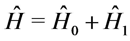 . The first term
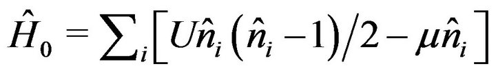 , with the onsite energy
  and the chemical potential
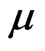 , describes the repulsion of more than one boson residing on a lattice site. It is local and diagonalizable in the occupation number basis for any lattice site. The second term
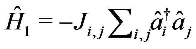 with the hopping matrix element
 if the lattice sites i and j are nearest neighbors and
  otherwise describes the hopping between two sites due to the quantum-mechanical tunneling effect. The competition between the two energy scales
  and J determines the existence of two different phases. When the on-site energy is small compared to the hopping amplitude, the ground state is superfluid (SF) as the bosons are delocalized in a phase coherent way over the whole lattice. In the opposite case, where the on-site interaction dominates over the hopping term, the ground state is a Mott insulator (MI) where each boson is trapped in one of the respective potential minima.
This characteristic quantum phase transition of the Bose-Hubbard model has been studied extensively both with analytical [5-11] and numerical [12-14] methods for zero temperature, while less literature exists on the finitetemperature properties of this transition [15-17]. In this letter we work out an analytical Green’s function approach in order to determine the MI-SF phase boundary and the excitation spectrum in the Mott phase both for zero and finite temperature with a hopping expansion. Our findings compare well with the latest findings of Quantum Monte Carlo simulations and allow to propose a thermometer for bosons in optical lattices. In the following we restrict ourselves to a spatially homogeneous system and neglect the effects arising from the additional harmonic confining potential, which is present in all experimental settings, like the formation of a shell structure [18]. However, these effects could be taken into account by applying the local density approximation where the external potential is taken into account in form of a spatially dependent chemical potential.
2. Green’s Function Approach
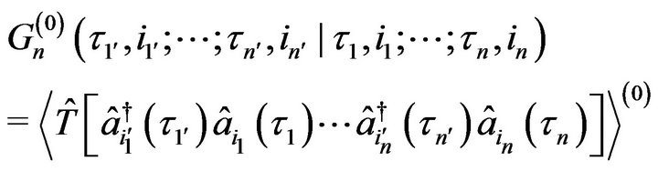
As all single-particle properties of a quantum many-body system are contained in its Green function, we base our calculation on this quantity. Because we are interested in describing a system at non-zero temperature, we use the imaginary-time formalism [19,20]. Therein, the singleparticle Green function is defined as the thermal average of the time-ordered product of a creation and an annihilation operator in Heisenberg representation
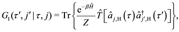 (1)
(1)
with ,
,  and we have introduced the partition function
 . Because it is not possible to obtain analytic expressions for the eigenstates and eigenenergies of the full Bose-Hubbard Hamiltonian, we can not calculate the Green function exactly. Instead, we aim at a perturbative treatment and calculate this quantity as a power series in the hopping matrix element
 . As that parameter is small for the Mott phase, where the lattices are deep and the interaction between particles is strong, we refer to this treatment as a strongcoupling expansion. In order to employ this perturbative expansion for finite temperature we make use of the Dirac interaction picture and write the imaginary-time evolution operator in form of a Dyson series,
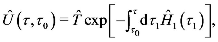 (2)
(2)
where the time dependence of the Dirac-picture operators is determined by the local Hamiltonian . With its help we can write the Green function as
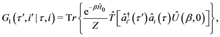 (3)
(3)
where the time-ordering operator acts also on the time variables which are resulting from the expansion of the Dirac imaginary-time evolution operator in (2). When we now expand perturbatively in powers of the tunneling matrix element J, the 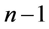 th order contribution
 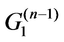 in (3) turns out to depend on the n-particle Green function of the unperturbed system as
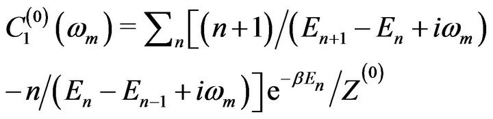
In order to determine 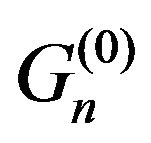 we cannot use standard Wick’s theorem because the unperturbed Hamiltonian
  is not quadratic in the Bose operators. Although the lack of Wick’s theorem in the present situation prevents us from using the powerful perturbative technique based on standard Feynman diagrams, we can nevertheless simplify
  by decomposing it into cumulants. To this end, we follow an approach reviewed by Metzner [21] in the context of the Hubbard model which describes electrons in a conductor. This decomposition is based on the important observation that the on-site Hamiltonian
  is local. Consequently, the unperturbed Green functions
  are also local and can be decomposed into timedependent cumulants
 . For instance, we have
  with the cumulant
 (4)
(4)
where  is the unperturbed partition function for a single-site system with the on-site energy eigenvalues
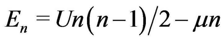 . With this decomposition, we can represent
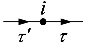
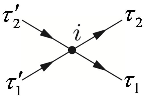
  diagrammatically: We denote an n-particle cumulant at a lattice site by a vertex with n entering and n leaving lines with imaginary-time variables, so we have, for instance, for the first two cumulants
 (5)
(5)
 . (6)
. (6)
Furthermore, the hopping matrix element is symbolized by a line connecting two vertices:
i j = Jij. (7)
With all this, we can set up the diagrammatic rules for calculating the n th order contribution of the Green function in J. First: Draw all possible combinations of vertices with total n internal and one entering and one leaving line. Second: Connect them in all possibles ways and assign time variables and hopping matrix elements to the lines. Third: Sum all site indices over all internal lattice sites and integrate all internal time variables from  to
to .
.
We also note here that we have to sum all site indices over the whole lattice, no matter whether two sites in a diagram coincide or not. We make use of the translational invariance in imaginary time and transform all expressions to Matsubara space. In the second diagrammatic rule the integrals over the time variables have to be replaced by sums over all bosonic Matsubara frequencies 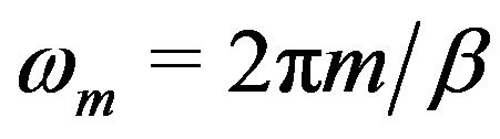 with integer m where the sum of the incoming frequencies must equal the sum of the outgoing ones.
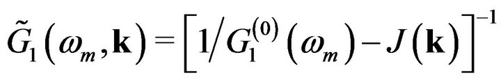
The formalism developed so far allows for calculating the Green function to any given order in the tunneling matrix element J. But because one of our main goals is to describe the phase transition between the Mott insulator and the superfluid phase, and it is well known in the theory of critical phenomena that such a transition is characterized by diverging long-range correlations [20,22], we must employ a non-perturbative method which is archieved by summing an infinite subset of diagrams. In order to perform this task, we introduce the sum of all one-particle irreducible diagrams including their respective symmetry factors and multiplicities as
 =
=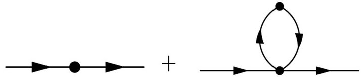 +··· (8)
The self-energy which describes the movement of a single particle in a many-body enviroment is defined as 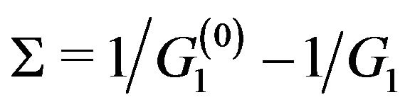 [19]. For our case, it can be written in the form
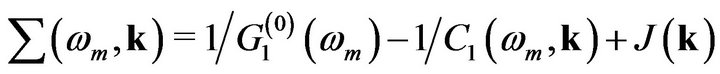 , where
 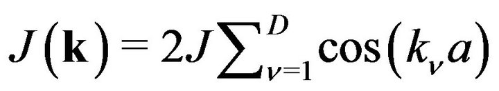 is the D-dimensional lattice dispersion. For instance, the first order in the self-energy which corresponds to a summation of all simple chain diagrams, yields
with
 .
.
We note that performing the limit  in the Green function allows to obtain the quasi-momentum distribution needed to explain experimental time-of-flight pictures [23-25].
3. Phase Boundary
The boundary of the phase transition is characterized by diverging long-range correlations [20,22]. Thus, we set  and solve for the value of J where the Green function diverges which is only possible for
 . This yields up to first order in J
 (9)
(9)
which coincides with the finite-temperature mean-field result [16,17,26]. The zero-temperature limit of (9), i.e.
 , agrees with the seminal mean-field result of Ref. [1]. The reason for this agreement is that each approximation becomes exact in the limit of infinite spatial dimension. In order to see that one must suitably scale the hopping parameter [27-29]. When we define
 , the contribution of the
  th order chain diagram is proportional to
  because there exist
  possibilities in a chain diagram for every hopping line to connect to neighboring sites. The lowestorder term neglected by that summation is the one-loop diagram in (8) which has two internal lines but only one free index and is, therefore, proportional to
  . Thus, it vanishes in the limit of
  .
.
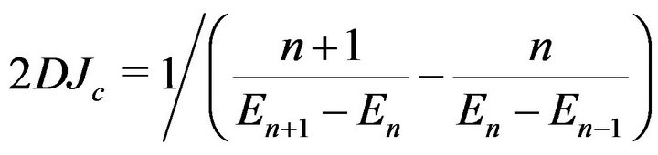
Taking now the one-loop diagram into account yields
 , (10)
where  is the second-order self-energy with the value of the one-loop diagram
 . The analytic formula for the phase boundary resulting from this formula is shown in Figure 1. This result coincides in the limit of
  with the effective potential formalism employed in Ref. [9]. We want to emphasize that, unlike the first order (9), the oneloop corrected result depends on the system dimension in an non-trivial way and that the corrections are larger in two than in three dimension which is consistent with the fact that the first-order results becomes exact in the limit
 . Note that even higher-order corrections for the effective potential formalism have been obtained in Refs. [10,11], which turned out to be indistinguishable from the Quantum Monte-Carlo data in Ref. [13].
For finite temperature, the phase boundary is shifted towards larger values of  as thermal fluctuations suppress quantum correlations which are responsible for the formation of the superfluid. This effect, which occurs both in first and in second order, is most important between the Mott lobes as fluctuations are strongest when the average particle number is not near an integer value. The correction to the mean-field result arising from the one-loop diagram, visible in the difference between first and second order curve, plays an important role only near the tip of the Mott lobe. This feature stems from the fact that quantum fluctuation are notably increased when the system approaches the quantum critical point at the tip of the lobe [4]. Thus, we can say the quantum phase dia-
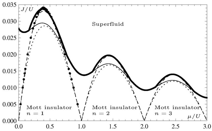
Figure 1. Quantum phase diagram for D = 3. Thick (solid): Second (first) order, kBT = 0.1U. Dashed (dotted): Second (first) order, T = 0. Dots: QMC Data for T = 0 [13].
gram consists of a thermally dominated region where the influence of thermal fluctuations is large and a quantum dominated region where the quantum corrections from the one-loop diagram are most important.
4. Excitation Spectrum
For a system in the Mott phase, three different types of excitations exist. 1) The addition of a particle from the environment (particle excitation); 2) The removal of a particle (hole excitation); 3) The creation of a particle-hole pair (pair excitation). The last one is most important from a physical point of view because it is also possible in an isolated system as realized in the current experiments. In the superfluid phase, there are additional excitations corresponding to fluctuations of the phase of the superfluid order parameter. However, these features can not be investigated within the present formalism but with the related effective action method [30].
In order to obtain the spectrum of the quasi-particles, which is given by the poles of the real-time Green function for finite temperature we must analytically continue our imaginary-time result. This is achieved by performing the replacement  with
with  [19]. The first and second order, respectively, yield excitation spectra of which the former one agrees in the limit
  with the mean-field result from Ref. [7]. In the following we restrict ourselves to the most interesting case
 . Both finite temperature and one-loop corrections are most effective for small wave numbers, the former because the effect of temperature is the suppression of quantum correlations which mainly exist for long wavelengths, the latter because the dominant fluctuations near a quantum critical point are the ones with vanishing wave number as shown in Figure 2.
All spectra show a characteristic gap which vanishes at the critical point, i.e. at the value of  at the tip of a Mott lobe. In Figure 3 its temperature dependence is shown. As this gap is a quantity which is experimentally accessible [18], it could serve as a method to determine the temperature of bosons in an optical lattice. The quasiparticle can be ascribed an effective mass which is shown in Figure 4 for the particleand for the hole-excitations. They both become massless at the critical point which is a result of the U(1) symmetry breaking at the secondorder phase transition.
5. Conclusion and Outlook
We have presented a powerful formalism to calculate the Green function for the Bose-Hubbard model in the Mott phase. It allowed us to improve the mean-field phase boundary in an analytic way both for finite and zero temperature where the former result deviates from recent Quantum Monte-Carlo studies by only 3% for  in
in
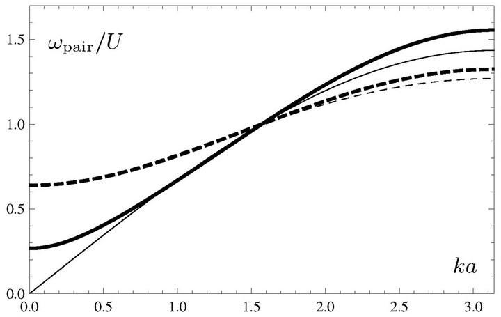
Figure 2. Dispersion relation of the pair-excitations for T = 0. Thick lines: second order; Thin lines: first order; Solid: J = 0.029U; Dashed: J = 0.025U.
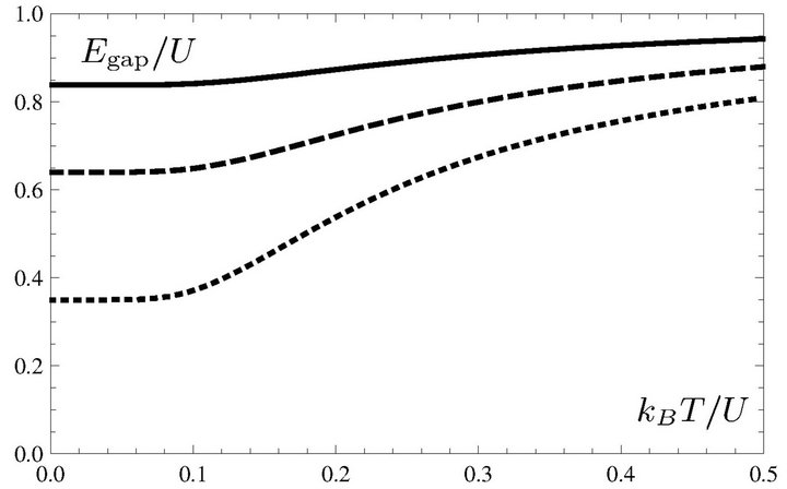
Figure 3. Temperatue dependence of gap for unit filling. Solid: J = 0.008U; Dashed: J = 0.012U; Dotted: J = 0.025U.
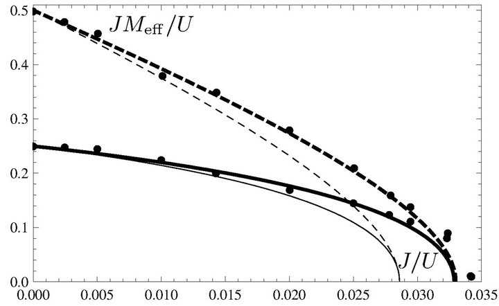
Figure 4. Effective masses of quasi-particles (solid lines) and quasi-holes (dashed lines) for T = 0. Thick lines: second order; Thin lines: first order; Dots: QMC data [13].
Ref. [13]. For finite temperature first analytic results beyond mean-field theory have been presented and the importance of both thermal and quantum fluctuations in the different regions of the phase diagram has been clarified. In addition, we have calculated the excitation spectrum of the quasi-particles and derived its effective masses and compared them to numerical findings. We have also investigated the characteristic energy gap and determined its temperature dependence. More applications of this approach have recently allowed in Ref. [31] to obtain more insight into the superfluid phase by combining the present technique with the effective action approach from Ref. [30].
6. Acknowledgements
We cordially thank B. Bradlyn, H. Enoksen, A. Hoffmann, H. Kleinert, F. Nogueira, R. Graham, and F. E. A. dos Santos for stimulating and helpful discussions.
REFERENCES
- M. P. A. Fisher, P. B. Weichman, G. Grinstein and D. S. Fisher, “Boson Localization and the Superfluid-Insulator Transition,” Physical Review B, Vol. 40, No. 1, 1989, pp. 546-570. doi:10.1103/PhysRevB.40.546
- D. Jaksch, C. Bruder, J. I. Cirac, C. W. Gardiner and P. Zoller, “Cold Bosonic Atoms in Optical Lattices,” Physical Review Letters, Vol. 81, No. 15, 1998, pp. 3108-3111. doi:10.1103/PhysRevLett.81.3108
- M. Greiner, O. Mandel, T. Esslinger, T. W. Hänsch and I. Bloch, “Quantum Phase Transition from a Superfluid to a Mott Insulator in a Gas of Ultracold Atoms,” Nature, Vol. 415, 2002, pp. 39-44. doi:10.1038/415039a
- S. Sachdev, “Quantum Phase Transitions,” 2nd Edition, Cambridge University Press, Cambridge, 2011.
- J. K. Freericks and H. Monien, “Strong-Coupling Expansions for the Pure and Disordered Bose-Hubbard Model,” Physical Review B, Vol. 53, No. 5, 1996, pp. 2691-2700. doi:10.1103/PhysRevB.53.2691
- N. Elstner and H. Monien, “Dynamics and Thermodynamics of the Bose-Hubbard Model,” Physical Review B, Vol. 59, No. 19, 1999, pp. 12184-12187. doi:10.1103/PhysRevB.59.12184
- D. van Oosten, P. van der Straten and H. T. Stoof, “Quantum Phases in an Optical Lattice,” Physical Review A, Vol. 63, No. 5, 2001, Article ID: 053601. doi:10.1103/PhysRevA.63.053601
- D. B. M. Dickerscheid, D. van Oosten, P. J. H. Denteneer and H. T. C. Stoof, “Ultracold Atoms in Optical Lattices,” Physical Review A, Vol. 68, No. 4, 2003, Article ID: 043623. doi:10.1103/PhysRevA.68.043623
- F. E. A. dos Santos and A. Pelsterr, “Quantum Phase Diagram of Bosons in Optical Lattices,” Physical Review A, Vol. 79, No. 1, 2009, Article ID: 013614. doi:10.1103/PhysRevA.79.013614
- N. Teichmann, D. Hinrichs, M. Holthaus, and A. Eckardt, “Bose-Hubbard Phase Diagram with Arbitrary Integer Filling,” Physical Review B, Vol. 79, No. 10, 2009, Article ID: 100503. doi:10.1103/PhysRevB.79.100503
- N. Teichmann, D. Hinrichs, M. Holthaus and A. Eckardt, “Process-Chain Approach to the Bose-Hubbard Model: Ground-State Properties and Phase Diagram,” Physical Review B, Vol. 79, No. 22, 2009, Article ID: 224515. doi:10.1103/PhysRevB.79.224515
- T. D. Kühner and H. Monien, “Phases of the One-Dimensional Bose-Hubbard Model,” Physical Review B, Vol. 58, No. 22, 1998, pp. R14741-R14744. doi:10.1103/PhysRevB.58.R14741
- B. Capogrosso-Sansone, N. V. Prokof'ev, and B. V. Svistunov, “Phase Diagram and Thermodynamics of the ThreeDimensional Bose-Hubbard Model,” Physical Review B, Vol. 75, No. 13, 2007, Article ID: 134302. doi:10.1103/PhysRevB.75.134302
- B. Capogrosso-Sansone, S. G. Söyler, N. Prokof'ev and B. Svistunov, “Monte Carlo Study of the Two-Dimensional Bose-Hubbard Model,” Physical Review A, Vol. 77, No. 1, 2008, Article ID: 015602. doi:10.1103/PhysRevA.77.015602
- H. Kleinert, S. Schmidt and A. Pelster, “Reentrant Phenomenon in the Quantum Phase Transitions of a Gas of Bosons Trapped in an Optical Lattice,” Physical Review Letters, Vol. 93, No. 16, 2004, Article ID: 160402. doi:10.1103/PhysRevLett.93.160402
- P. Buonsante and A. Vezzani, “Phase Diagram for Ultracold Bosons in Optical Lattices and Superlattices,” Physical Review A, Vol. 70, No. 3, 2004, Article ID: 033608. doi:10.1103/PhysRevA.70.033608
- K. V. Krutitsky, A. Pelster and R. Graham, “Mean-Field Phase Diagram of Disordered Bosons in a Lattice at Nonzero Temperature,” New Journal of Physics, Vol. 8, 2006, p. 187. doi:10.1088/1367-2630/8/9/187
- S. Fölling, A. Widera, T. Müller, F. Gerbier and I. Bloch, “Formation of Spatial Shell Structure in the Superfluid to Mott Insulator Transition,” Physical Review Letters, Vol. 97, No. 6, 2006, Article ID: 060403. doi:10.1103/PhysRevLett.97.060403
- A. A. Abrikosov, L. P. Gorkov and I. E. Dzyaloshinski, “Methods of Quantum Field Theory in Statistical Physics,” Dover Publications, New York, 1963.
- J. Zinn-Justin, “Quantum Field Theory and Critical Phenomena,” 4th Edition, Oxford University Press, Oxford, 2002. doi:10.1093/acprof:oso/9780198509233.001.0001
- W. Metzner, “Linked-Cluster Expansion around the Atomic Limit of the Hubbard Model,” Physical Review B, Vol. 43, No. 10, 1993, pp. 8549-8563. doi:10.1103/PhysRevB.43.8549
- H. Kleinert and V. Schulte-Frohlinde, “Critical Properties of Φ4-Theories,” World Scientific, Singapore, 2001. doi:10.1142/9789812799944
- F. Gerbier, et al., “Phase Coherence of an Atomic Mott Insulator,” Physical Review Letters, Vol. 95, 2005, Article ID: 050404. doi:10.1103/PhysRevLett.95.050404
- A. Hoffmann and A. Pelster, “Visibility of Cold Atomic Gases in Optical Lattices for Finite Temperatures,” Physical Review A, Vol. 79, No. 5, 2009, Article ID: 053623. doi:10.1103/PhysRevA.79.053623
- F. Gerbier, S. Trotzky, S. Foelling, U. Schnorrberger, J. D. Thompson, A. Widera, I. Bloch, L. Pollet, M. Troyer, B. Capogrosso-Sansone, N. V. Prokof’ev and B. V. Svistunov, “Expansion of a Quantum Gas Released from an Optical Lattice,” Physical Review Letters, Vol. 101, No. 15, 2008, Article ID: 155303. doi:10.1103/PhysRevLett.101.155303
- F. Gerbier, “Boson Mott Insulators at Finite Temperatures,” Physical Review Letters, Vol. 99, No. 12, 2007, Article ID: 120405. doi:10.1103/PhysRevLett.99.120405
- W. Metzner and D. Vollhardt, “Correlated Lattice Fermions in d = ∞ Dimensions,” Physical Review Letters, Vol. 62, No. 3, 1989, pp. 324-327. doi:10.1103/PhysRevLett.62.324
- L. Amico and V. Penna, “Dynamical Mean Field Theory of the Bose-Hubbard Model,” Physical Review Letters, Vol. 80, No. 10, 1998, pp. 2189-2192. doi:10.1103/PhysRevLett.80.2189
- K. Byczuk and D. Vollhardt, “Correlated Bosons on a Lattice: Dynamical Mean-Field Theory for Bose-Einstein Condensed and Normal Phases,” Physical Review B, Vol. 77, No. 23, 2008, Article ID: 235106. doi:10.1103/PhysRevB.77.235106
- B. Bradlyn, F. E. A. dos Santos and A. Pelster, “Effective Action Approach for Quantum Phase Transitions in Bosonic Lattices,” Physical Review A, Vol. 79, No. 1, 2009, Article ID: 013615. doi:10.1103/PhysRevA.79.013615
- T. D. Grass, F.E.A. dos Santos and A. Pelster, “Excitation Spectra of Bosons in Optical Lattices from the Schwinger-Keldysh Calculation,” Physical Review A, Vol. 84, No. 1, 2011, Article ID: 013613. doi:10.1103/PhysRevA.84.013613