Atmospheric and Climate Sciences
Vol.05 No.02(2015), Article ID:55722,14 pages
10.4236/acs.2015.52007
Changes in Environmental Parameters and Their Impact on Forest Growth in Northern Eurasia
Olga Khabarova1, Igor Savin2
1Heliophysical Laboratory, The Pushkov Institute of Terrestrial Magnetism, Ionosphere and Radiowave Propagation RAS (IZMIRAN), Moscow, Russia
2V.V. Dokuchaev Soil Science Institute, Moscow, Russia
Email: habarova@izmiran.ru
Copyright © 2015 by authors and Scientific Research Publishing Inc.
This work is licensed under the Creative Commons Attribution International License (CC BY).
http://creativecommons.org/licenses/by/4.0/


Received 24 March 2015; accepted 9 April 2015; published 16 April 2015
ABSTRACT
We performed an empirical investigation of forest growth for two types of forests in northern Eurasia (larches and spruces) in order to show that the sensitivity of trees to the variable climate and geomagnetic field can be seen even under the large-scale average. The main purpose of this research was to model a forest growth rate V for each forest type on the basis of several environmental parameters influencing the tree growth in a high degree and to find the differences and similarities of the larches and spruces’ response to changing environment. We showed that V, which is related to the annual tree-ring width, could be derived from the Normalized Difference Vegetation Index (NDVI) data. Averaged yearly by species for 1982-2006, it displayed a long-term decrease (most likely related to the global climate change) as well as short-term variations with periods of 2.2, 4 and 8 years. A composite function method was used for modeling. We selected several tree growth drivers (the temperature, precipitation, insolation and the geomagnetic field intensity) that were highly correlated with V, and a function was modeled that described the behavior of V. The correlation coefficients between the derived function and experimental time series were 0.8 for larches and 0.9 for spruces. Compared with spruces, larches demonstrated higher thermo-sensitivity. A loss of tree sensitivity to temperature changes is puzzling for dendroclimatology, as a similar process might have occurred during previous periods of sharp global climate changes (as observed currently). Sensitivity of trees to geomagnetic field changes is confirmed both at long- and short-timescales. Spruces are found to be more magnetosensitive than larches.
Keywords:
Climate Change, Forest Growth, Biomagnetism

1. Introduction
Recent decades have been characterized by significant climate changes and consequent changes in terrestrial ecosystems, particularly forests. The normal functional conditions of many biotic components appear to be disordered on both local and regional scales. This is reflected in stress-induced tree mortality and tree growth degradation [1] -[3] . Even moderate environmental changes have produced visible shifts in forest vegetation dynamics, which have been detected by geostationary operational environmental satellites. Remote sensing, the most general method for observing the biosphere, allows the monitoring of climate-related changes in forest productivity (or greenness). Greenness can be successfully estimated through special indices such as the Leaf Area Index (LAI), Vegetation Optical Depth (VOD) and Normalized Difference Vegetation Index (NDVI) [4] -[6] .
The number of reports on negative changes in forest homeostasis (if to consider trees as an organism) increases every year. However, there have also been reports of the locally successful adaptation of forests to observed environmental changes as well as positive tendencies in the growth of certain species such as oaks [7] [8] . Therefore, certain questions arise:
-Do the environmental changes of recent decades influence forests negatively or positively?
-Can we estimate the global impact of climate changes on trees, or is the effect obvious only at local scales?
-Can we find an empirical model (formula) that satisfactorily represents the observed changes in forest growth at global scale?
In answering these questions, we should analyze observational data on the green biomass volume for large areas and define environmental parameters that determine forest development.
Parameters such as precipitation, insolation and temperature, are used in different forest simulation models. They are typically considered to be forest growth determinants (see [9] [10] and references therein, as well as links at http://models.etiennethomassen.com). The problem is that an ecosystem cannot be satisfactorily described by a linear model because the involved dependences are very complex. For example, the thermal sensitivity of ecosystems was experimentally found to be constant and independent of other environmental factors [11] , in contrast with several predictive models. Even nonlinear models that consider exponential thermal dependence of plant growth and plant respiration have several problems that are possibly related to neglected thermal acclimation [12] .
Thus, our model should be nonlinear and include several parameters that influence tree growth to a substantial degree. Three of these parameters are well known and are mentioned above. However, there is an additional, often underestimated, parameter that should also be included in our tree growth model as an additional environmental component: a magnetic field.
Trees are a conductive medium containing moving liquid to which all electromagnetic effects may be applied. Like animals, trees demonstrate their ability to be magneto-sensors. The sensitivity of plants and trees to electromagnetic fields (both from natural and artificial sources) has been investigated by specialists in various countries for many years. There is evidence of plant and tree responses to magnetic field changes. This includes magnetotropism, sensitivity to variations of the geomagnetic and artificial magnetic fields in ultra-low-frequency diapason, plant reactions to magnetic storms, and many other effects (see [13] -[18] and references therein).
Although it represents a second-order effect, there are several practical applications of plant magnetosensitivity. For example, the stimulation of plant productivity and growth by a pulsing magnetic field was widely used in the USSR as a method to increase crop yields [19] -[22] . Recent investigations have confirmed previously obtained results and shown new possibilities for the treatment of plants with magnetic fields [15] [23] -[25] .
Natural variations in the Earth’s magnetic field may impact plants and trees both directly and indirectly (for instance, through variations in the atmospheric electric field). The latter effect will be discussed below, and the first effect is determined by Ampere’s law and the Lorentz force applied to sap (or any other biological liquid) as well as by mechanisms of forced and parametrical resonances in bio-objects [26] -[32] . Therefore, it would be reasonable to analyze a “tree growth-geomagnetic activity index changes” relationship based on a large-scale approach.
In the current investigation, we do not consider the direct impact of CO2 on forest productivity [33] , as it is difficult to observe carbon fluxes at the global scale, and we assume this parameter to be dependent on the above-mentioned environmental factors. The aim of this paper is to analyze the “forest growth-environmental changes” connection at the global scale.
The main idea of our investigation may be stated as follows: if consequences of climate change are observed locally in many places, then the response of trees should also be visible in large-scale averages. The response of forests to a variable environment was studied based on remote sensing data for the annual biomass volume gained by larches and spruces in northern Eurasia over a period of 25 years. We averaged the NDVI by species and calculated a yearly tree growth rate as a function of NDVI. The tree growth rate was simulated on the basis of key environmental parameters. We demonstrated the importance of incorporating the cumulative effects of various contributing factors (including the geomagnetic field) that determine the vegetation activity of trees.
2. Methods
2.1. General Approach
For our purposes, we have to find a proper method for estimating the global-scale dependence of tree growth on climate change and for modeling the growth of forests in northern Eurasia. A method in which correlative maps are used to examine global-scale forest productivity appears to best meet this requirement [34] -[37] . According to this method, the world map is divided into grids measuring several square kilometers (pixels on the map), where some vegetation index X such as LAI or NDVI and a climatic variable Y (such as air temperature and atmospheric pressure) are recorded for a reasonably long time t. Both X and Y are averaged over each pixel with a time step Dt << t. A correlation coefficient between the X and Y time series is then calculated for the same time interval (month, season, year, etc.) for every grid. As a result, a color map of correlation coefficients, which are marked with colors corresponding to values from −1 to +1, is obtained. This map is used as an alternative to visual comparative analysis of climate and vegetation maps (one map is analyzed instead of two).
Islands of a dominant color are easily observed on correlative maps, exposing areas of quasi-stable positive/ negative strong relations between vegetation characteristics and climatic parameters and allowing the estimation of long-term trends in the revealed relationships. The effectiveness of such an approach was shown in [38] and [39] . The approach was used to study correlations between LAI and the El Niño southern oscillation [38] as well as between NDVI, temperature and precipitation in northern and southern semiarid regions [39] .
Therefore, the method is appropriate for showing climate-vegetation dependencies in a large-scale study. However, the method does have certain limitations, because correlation coefficients vary from −1 to 1, and areas of dominant positive/negative correlation are local. If the coefficients are averaged over the entire map, no correlation may be found between the examined variables, as even adjacent areas of several tens of square kilometers may be characterized by different vegetation trends.
For example, the linear trend in LAI calculated for 1982-1990 was significantly positive in Europe, Siberia and many other large-scale areas, but negative in central and western Canada [40] . Climate change leads to a variability of correlation coefficients between vegetation and climatic indices through the map, as demonstrated by Buermann et al. [38] , who analyzed global LAI variations in comparison with El Niño events. South-central and southeastern South America and southwestern Africa showed positive correlations of LAI with the El Niño NIÑO3 index, whereas eastern Australia, northeastern Brazil, southeastern and central Africa, Indonesia, Central America and the west coast of the United States were characterized by negative correlation coefficients. There were also vast areas on the globe with zero correlation between LAI and NIÑO3 [38] .
Thus, if one averages correlation coefficients, for example, for the pair “NDVI―air temperature” over the entirety of northern Eurasia, the result is approximately zero for any time interval used for averaging. However, this result does not indicate the absence of global climate impact on tree growth because strong relationships between climate changes and tree growth are indeed observed. Hence, the discussed method must be modified to show correlations between vegetation characteristics and climate variables under global averaging.
We suppose here that an apparent “zero result” in correlation mapping may be avoided by separating species, that is, through the use of vegetation indices that characterize the greenness level of particular types of trees. We do not use the ordinary multi-species NDVI but, rather, an index associated with a certain species. Such an approach might yield a positive outcome in view of the result obtained by Bowman and Prior [41] , who showed that a general continental-scale growth trend of certain species occurs irrespective of the climate zone.
2.2. Selection of Species, Habitats and Basic Data for Investigation
The Northern Eurasian region was selected for the study, as demonstrated in Figure 1 (after [42] ). Types of vegetation are indicated through the analysis of the seasonal dynamics of NDVI [42] .

Figure 1. Locations of the analyzed areas in northern Eurasia. The areas covered by evergreen trees are shown in green, and deciduous larch forests are shown in brown.
Additional information on the vegetation map preparation can be found at http://bioval.jrc.ec.europa.eu/products/glc2000/products.php. According to the map, coniferous deciduous (larches, Larix) and coniferous evergreen (spruces Pícea, Abies, Pinus) forests cover, respectively, 8,032,392 km2 and 4,785,994 km2 of northern Eurasia (brown and green areas in Figure 1). As remote sensing is one of the best methods for the global observation of terrestrial surface and atmospheric processes [43] , we have used National Oceanic and Atmospheric Administration (NOAA) Advanced Very High Resolution Radiometer (AVHRR) meteorological satellite NDVI data (see data and documentation at http://gimms.gsfc.nasa.gov/ndvi/ndvie/GIMMSdocumentation_NDVIe.pdf). The index has a spatial resolution of ~64 km2 and a temporal resolution of 15 days. We calculated yearly NDVI for 25 years (1982-2006) for both evergreen and deciduous trees over the regions shown in Figure 1 in order to examine tree-climate relationships at the large scale.
2.3. Parameters Used for Analysis
As we are interested in forest growth estimation and simulation, the most appropriate parameter for this purpose is the yearly forest growth rate. This parameter can be derived from NDVI characteristics similar to [44] . Figure 2 represents the typical behavior of NDVI during one year. The ordinate of the maximum of the NDVI curve divided by the growing season length t, as shown in Figure 2, gives an approximate average yearly tree growth speed (rate) V, multiplied by two:
 , (1)
, (1)
where tmax is the time at which NDVI reaches its maximum. It follows from Equation (1) that the dimension of V is [NDVI arbitrary units/days]. Note that this parameter correlates with the rate of tree-ring yearly radial growth (annual tree-ring width), which is a key point for dendro-ecological and dendro-climatological studies [45] . Satellite data are widely used to assess plant production by linking the amount of absorbed photosynthetically active radiation with gross primary productivity (the total biomass). At the same time, the cambium material of tree rings is a product of photosynthesis; therefore, the linkage between remote sensing indicators of forest productivity and variations in tree ring width is logical. From this perspective, it is not surprising to find a positive association between NDVI and tree ring measurements, as demonstrated in many previous studies [45] -[50] .
The most influential external factors for the selected tree species were then determined and compared with V. We analyzed different environmental parameters that were averaged yearly for the entire areas covered by deciduous and evergreen forests. We then selected several environmental parameters from all possible ones (both mentioned above and such as cloudiness, ultraviolet index, wind speed, etc.), considering only the highest and statistically significant values of correlation coefficients between V and the examined parameters (see Results). These parameters are as follows:
1) Sum of incoming radiation per growing season: F (W/m2);
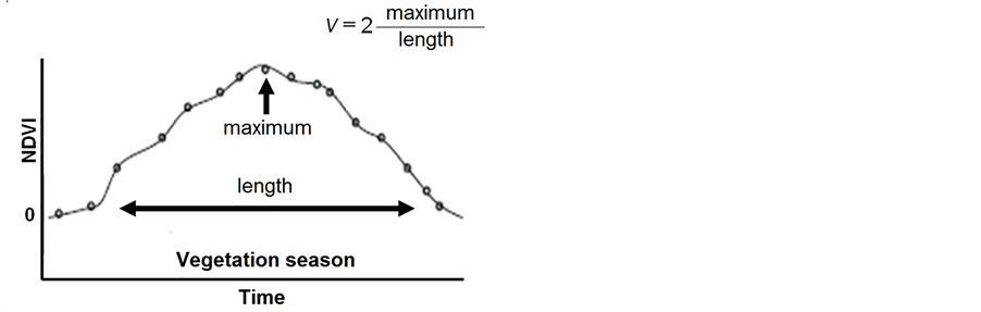
Figure 2. Parameter characterizing annual forest growth. The yearly achieved NDVI maximum is divided by half of the growing season length. The parameter represents the yearly mean rate of green biomass gain (the forest growth rate).
2) Relative irradiation, which is F per growing season of t days length:  (W/m2 days). Days should be multiplied by 15 (as the NDVI measurement resolution is 15 days);
3) Mean temperature per growing season: T (˚C);
4) Yearly amount of precipitation: P (kg/m2);
5) Annual value of the Kp index of geomagnetic activity: Kp.
Parameters F, F¢ and P were obtained from the ECMWF ERA Interim archive (http://www.ecmwf.int/products/data/archive/descriptions/ei/index.html) and calculated for the areas covered by each considered species.
The Kp index, which characterizes geomagnetic activity variations at the global scale, is a 3-hour index calculated on the basis of data from 13 magnetometric observatories located over the globe (see an explanation of the index derivation at http://www.wdc.rl.ac.uk/Help/Kp/Derivation.html, and data at http://omniweb.gsfc.nasa.gov/form/dx1.html). The yearly averaged Kp index adequately represents the change in geomagnetic activity level under a multi-year analysis.
2.4. Method Used for Modeling
A composite function method was used as an empirical modeling technique, analogous to the neural network method (a description can be found in reference [51] ). This nonlinear method helps to reach the maximum of correlation between one dependent and several independent time series, if there is a real cause-effect relation between the series. In such a case, independent parameters, taken separately, are usually only moderately correlated with a variable, but their optimal combination could give a higher correlation with the variable.
The first step is a correlation analysis. Most strongly correlated time-series are identified (the modeled variable is supposed to be dependant). The positively correlated parameters are placed in the numerator, and the negatively correlated parameters are placed in the denominator. A simple linear correlation analysis does not allow the consideration of complex mutual dependences of different climatic factors and cannot describe the nonlinear reaction of a species to this environmental “cocktail”. Therefore, a simulation is performed according to the algorithm discussed below.
Expert evaluation is an important part of the next step. An expert should test the most plausible view of the dependences between the analyzed parameters. Thus, the method demands a broad knowledge of the nature of the simulated processes. The last step is the adjustment of the computer coefficients, which can be demonstrated using the example of the row bn (where ).
).
We now determine the best bn view for the linear combination of K independent rows,
 (2)
(2)
with coefficients  that are determined by the condition that the maximal correlation between the fitting parameter and rows
  should be obtained:
 (3)
(3)
In this case, the coefficients should produce a maximum of the criterion function:
 (4)
(4)
where  and
and  are estimates of the cross-correlations between the factors. If factors
  and
and  are statistically independent and as small as
 , then the maximum is achieved at
  and equals
 (5)
(5)
3. Results
3.1. Correlation and Fourier Analysis
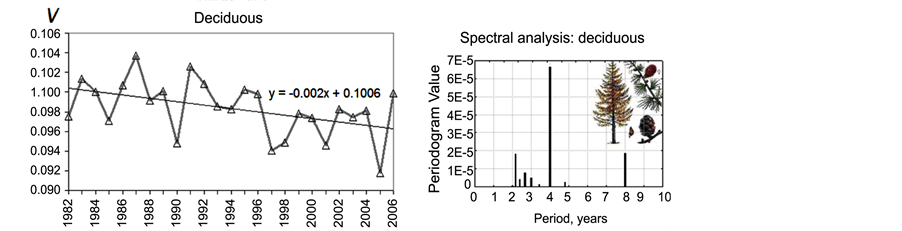
The time series of the yearly rate of tree growth V observed for deciduous and evergreen forests are shown in Figure 3(a) and Figure 3(b), respectively. First, there is a visible decreasing trend in V for both types of forests, possibly related to global climate change. Forests demonstrate the remarked decrease in the growth rate. For example, in the case of spruces, the approximation line crosses the axis of abscises within the next 244 years (the formula of linear approximation is indicated above the curve in Figure 3(b)). This means that if the current trend continues and the adaptation limit is surpassed, spruce forests in Northern Eurasia are in danger of extinction.
In addition to the long-term trend, relatively short variations in forest productivity with periods of several years are observed. A spectral analysis of the V time series is given in Figure 3(c) and Figure 3(d). The most evident periods are 2.2, 4 and 8 years for both deciduous and evergreen forests and 4.8 years for evergreens.
 (a) (c)
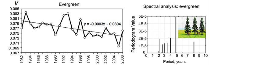 (b) (d)
Figure 3. Variations in forest growth rate and its spectral analysis. The forest growth rate V time series for larches (a) and spruces (b). Spectral analysis results for larches (c) and spruces (d).
Such variations are most interesting to consider because they reflect the sensitivity of trees to the variable environment.
As mentioned above, the first step of modeling was the selection of parameters. All parameters listed in Subsection 2.3. “Parameters used for analysis” were considered as possible candidates among other variables such as winter precipitation, number of sunspots and cloudiness. Figure 4 represents the results of a correlation analysis of V with the five environmental parameters that demonstrated the highest correlation coefficients. The correlation coefficients obtained for deciduous and evergreen forests are shown as gray and white boxes, respectively.
For the analyzed number of cases, statistically significant correlations at the one-tailed significance level of 0.05 should be at least 0.34. From this perspective, the correlations with T and Kp appear not to be as well established as those with the other parameters. However, we considered the known weak sensitivity of NDVI to temperature and artificially high sensitivity to precipitation [52] and decided to consider all of the parameters in Figure 4 for modeling.
The correlation coefficients are approximately the same for both deciduous and evergreen forests, with the exception of the response of trees to temperature changes. Spruces demonstrate a lack of thermosensitivity and a high dependence on relative insolation.
3.2. Simulation of Tree Growth Rate
From the various modeling functions representing the behavior of the original V time series, the most effective modeling parameter Vm was determined:
 . (6)
. (6)
This parameter is valid for both types of trees (Z = deciduous, evergreen). Its numerical coefficients C are shown in Table 1.
Equation (6) and Table 1 improve our understanding of several forest-climate complex connections. For example, geomagnetic field variations are an important influencing factor for evergreen trees because the input of the Kp term in Equation (6) is one order greater than the input of the term characterizing the temperature effect (see Table 1). At the same time, larches demonstrate a high sensitivity to temperature changes. Such effects are only a part of the entire nonlinear response of northern Eurasian forests to environmental changes described by Equation (6).
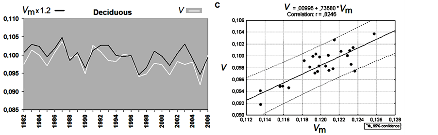
The validation of Equation (6) is shown in Figure 5. The experimental V time series are shown in white, and
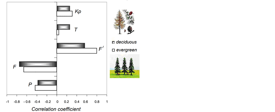
Figure 4. Coefficient of linear correlation between V and the environmental parameters that determine tree growth. Kp is the index of geomagnetic activity, T is the mean temperature for the growing season, F and F¢ are irradiation and relative irradiation, respectively, per growing season, and P is precipitation.
the modeling parameter Vm, calculated for both deciduous and evergreen forests, is represented by the black lines in Figure 5(a) and Figure 5(b). A remarkably high correlation is observed between Vm and V. The correlation coefficients are 0.83 and 0.92 for deciduous and evergreen forests, respectively, as shown in the scatterplots on the right side of the corresponding figures (Figure 5(c) and Figure 5(d)).
These correlation coefficients are greater than the correlation coefficients between V and the analyzed parameters, separately included in Equation (6), by |0.1 - 0.5|, which demonstrates the success of the modeling and confirms our hypothesis of the possibility of revealing the combined impact of environmental parameters on forests.
4. Discussion
In this study, we have emphasized the importance of considering a combination of different environmental drivers to better understand the dynamics of bio-systems. In particular, forests demonstrate sensitivity to various external variables, which might be taken into account altogether. A large-scale approach to the investigation of tree growth in northern Eurasia and its dependence on the changing environment has yielded unexpected as well as expected results.
The expected results are as follows:
 (a) (b)
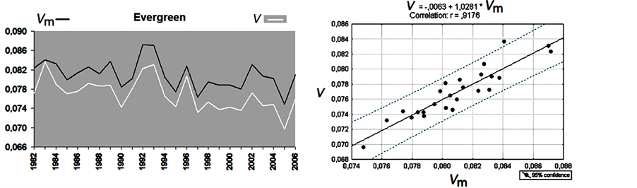 (c) (d)
Figure 5. Results of modeling. Vm is a simulated parameter, and V is the observed tree growth rate for deciduous (a) and evergreen forests (b) in northern Eurasia. The corresponding regression lines and correlation coefficients are shown in the right panels, (c) and (d).

Table 1. Coefficients in Equation (6) for deciduous and evergreen forests (North Eurasia).
1) Trees are sensitive to climate changes (as is obvious even at large-scales);
2) The tree growth rate V can be simulated based on key environmental parameters;
3) “Forest growth―environment” connections are nonlinear.
However, there are rather unexpected results:
1) We have obtained a unified formula that describes the growth of different types of trees, meaning that different species demonstrate similar behaviors that depend on the same key environmental factors.
Different types of trees have different preferred environmental conditions, and it would be logically to find that completely different combinations of environmental variables were responsible for growth of spruces and larches. In other words, formula (6) is expected to have different view for different species. However, the examined species demonstrate a similarity in their adaptive characteristics. The coefficients in Equation (6) are different for these species, which corresponds to the adaptive “tuning” of spruces and larches to environmental changes against the background of their similar response to extreme conditions such as heat and cold waves, droughts and prolonged rainfalls.
2) Forest productivity depression is observed for both types of trees but is expressed most notably for spruces.
If the observed large-scale forest productivity trend continues, spruce forests will become extinct in northern Eurasia within the next 240 years. This statement is not a prediction (as the adaptation process is not considered) but an issue for environmental awareness as well as a topic for further investigations. Similar negative trends have been observed for different types of trees worldwide, and all projections of future climate have suggested severe reductions in tree growth [53] . Certainly, the real development of forest distributions depends strongly on a future climate warming scenario [54] , but the agreement among the results obtained by a number of different investigators is a sign of the negative impact of climate change on the biosphere.
3) Tree growth is a function of geomagnetic activity.
The geomagnetic sensitivity of trees has often been reported. Surprisingly, the Kp index of geomagnetic activity is correlated with V and may be used for forest growth modeling. The nature of this phenomenon is primarily related to the impact of magnetic fields on electrical processes in trees.
Plants are known to generate various types of intracellular and intercellular electrical signals in response to environmental changes [55] ; this phenomenon occurs not only in ‘sensitive’ plants (such as Mimosa pudica or Dionaea muscipula) but also in ordinary species [56] [57] . Variations in natural electromagnetic fields may change the velocities of these small-scale processes and impact trees as a whole.
The atmospheric electric field is the most important source of the electromagnetic sensitivity of trees [58] . The Earth’s atmosphere represents a dielectric medium between two plates of a capacitor: the positively charged ionosphere and the negatively charged ground. The vertical atmospheric electric field is approximately 100 to 200 volts per meter under the so-called fair weather condition [59] [60] . Thus, there is a strong potential difference between the root and the crown of a tree. The ground, which absorbs an unlimited amount of current, is a commonly used return path for electric currents. Therefore, trees and plants represent grounded conductors inside the capacitor.
Conductivity measurements of plant sap have been performed since the beginning of the 20th century [61] . Recent papers on the investigation of sap flow variations and electric potential variations in tree trunks have demonstrated advanced approaches to experimental planning and considered many influencing environmental factors [62] . Experiments with different species confirm the presence of difference of electric potentials inside plants and trees from a few millivolts to a few hundred millivolts, depending on the object’s height, temperature, soil characteristics and sap conductivity [63] [64] . Electric currents of several microamperes flow through trees during the fair weather condition and may be significantly larger during thunderstorms [62] [64] .
In certain places, the atmospheric electric field varies with the time of day and season according to the so- called “Carnegie curve” [65] and is very sensitive to cloudiness, illumination, humidity, dust, ionospheric conditions and global geomagnetic field changes (magnetic storms) [66] -[68] . The natural variations of the atmospheric electric field disappear inside buildings. This principle should be considered in planning indoor experiments with plants. This phenomenon was confirmed by the results of an interesting experiment performed indoors for a potted Ficus benjamina tree [69] . The experiment did not display any correlation between the “voltage and time of day, illumination, sap flow, electrode elevation, or ionic composition of soil”, in contrast with outdoor experiments.
Unfortunately, measurements of the electric field of the atmosphere are provided by several scientific groups in a very limited number of places in the world, so there are still no experiments featuring simultaneous measurements of the electrical characteristics of trees and atmospheric electricity. Such comparisons would be important, because a sudden impulse of the geomagnetic field associated with the beginning of any geomagnetic storm results in abrupt changes in the ionosphere and, consequently, in the atmospheric electric field [70] [71] . The atmospheric electric field significantly changes, too, during strong geomagnetic storms. The intensity of those changes depends on the local time and latitude, but sometimes geomagnetic field storms may be clearly traced in the electric potential variations of trees.
One example of this effect is shown in Figure 6. The measured tree (Populus nigra) electric potential (after 4 Figure 8 from reference [62] ) changes abruptly in accordance with the storm-time variations in the geomagnetic field, as shown in Figure 6(a) and Figure 6(b). The severe geomagnetic storm in this example produced a very strong change in the vertical component of the atmospheric electric field, which leads to pronounced changes in the electrical characteristics of trees.
This particular magnetic storm was unique because of its intensity [72] . Typically, magnetic storms are characterized by a Dst index level < −30 nT, and storms with Dst values below −100 nT are considered to be severe. The intensity of the geomagnetic field impacting trees during this period was one order of magnitude greater than usual.
Detailed experiments such as those reported in reference [62] are extremely rare, and the mechanism of the response of trees to changes in electromagnetic fields is still poorly understood and demands further investigations. However, certain reactions of plants and trees to geomagnetic field variations have been demonstrated. Therefore, it is reasonable to include parameters that characterize geomagnetic field intensity variations in models that describe tree growth and variation in leaf area indices.
As shown in Figure 4 and Table 1, spruces are most sensitive to geomagnetic field changes. An increased level of geomagnetic activity is a positive factor for spruces. Further investigations should provide a better understanding of the magnetosensitivity of different species.
1) The thermal sensitivity of trees depends on the species and is unexpectedly low for spruces.
This statement is in a good agreement with results [73] , which demonstrate that phenological sensitivity to temperature is very similar between Pyrénées and Fontainebleau forests, i.e. that thermal sensitivity of trees de- pends on species rather than on location.
During the considered period, spruces in northern Europe were substantially unaffected by temperature changes, whereas larches showed relatively strong effects. This difference may be an indicator of the strongly adaptive

Figure 6. Electric potential variations of trees during one of the most intense magnetic storms of the century. (a) Electric potential of a standing tree (electrode E11, Figure 8 from [62] ); (b) Dst-index of geomagnetic activity.
characteristics of evergreens. The poor correlation between temperature and evergreen growth is a puzzle for dendroclimatology, as spruces are believed to be thermo-sensitive. Theoretically, the radial growth of trees should depend on the summer temperature. However, a decreased thermal response of radial tree growth during recent decades has been reported by several authors [74] [75] . Most likely, global warming and the related CO2 increase are responsible for this effect. Indeed, increased CO2 may give additional “feeding” to trees and protect them from the effects of potentially stressful temperatures. This effect, called CO2 fertiliztion, was discussed in [76] .
It is quite probably that several periods of similar thermo-sensitivity loss have occurred in the past. This finding means that the results of dendroclimatological paleo-reconstructions may contain significant errors related to the discussed effect. This conclusion is consistent with the results of the recent work [77] in which serious biases in tree-ring climate proxies were reported.
5. Conclusions
1) Trees sensitivity to climate changes is obvious even under the rough spatial average if to examine a certain species, which confirms the idea that the typical response of certain species to environmental changes is the same irrespectively of the habitat.
2) The tree growth rate is a nonlinear function of variables which represent the “environmental cocktail”. These are the temperature, precipitation, insolation and the geomagnetic field intensity. Different species demonstrate similar behaviors that depend on the same key environmental factors.
3) The geomagnetic field most probably influences trees through variations of the atmospheric electric field. This is a secondary order effect.
4) Forest productivity depression is observed for both types of trees. Under reduced tree adaptation, this may lead to loss of vast areas covered by spruces in the relatively near future.
5) The thermal sensitivity of spruces was found to be unexpectedly low, which probably is a sign of changing amplitude of trees’ response to temperature variations. This may make a puzzle for dendroclimatology, which is based on a supposition of stable dependence between atmospheric temperature and yearly tree-ring width.
As a whole, our approach confirms that the tree response on environmental change may be examined under consideration of several key external factors determining tree growth. The latter can be easily estimated on the basis of NDVI (or other similar indices) data for the certain species averaged over the large area. Potentially, the discussed method can be applied to analysis of ecological hazards for the certain kind of trees at the regional level.
Acknowledgements
ECMWF ERA Interim archive data (http://www.ecmwf.int/products/data/archive/descriptions/ei/index.html) were used to derive the environmental parameters. The NDVI data are taken from NOAA websites (http://gimms.gsfc.nasa.gov/ndvi/ndvie/GIMMSdocumentation_NDVIe.pdf and http://www.cpc.ncep.noaa.gov/data/indices/sstoi.indices, respectively). The study was supported by the Russian Academy of Science program no. 28 “Problems of the Earth’s life origination and development” and partially by RFBR grant no. 13-9536-3398. We thank the unnamed reviewer for useful comments.
References
- Myneni, R.B., Keeling, C.D., Tucker, C.J., Asrar, G. and Nemani, R.R. (1997) Increased Plant Growth in the Northern High Latitudes from 1981 to 1991. Nature, 386, 698-702. http://dx.doi.org/10.1038/386698a0
- Bowman, D.M. (2009) Australia and Global Change. In: Cuff, D.J. and Goudie, A.S., Eds., The Oxford Companion to Global Change, Oxford University Press, New York, 48-52.
- Adams, H.D., Macalady, A.K., Breshears, D.D., Allen, C.D., Stephenson, N.L., Saleska, S.R., Huxman, T.E. and McDowell, N.G. (2010) Climate-Induced Tree Mortality: Earth System Consequences. EOS Transactions AGU, 91, 153-154. http://dx.doi.org/10.1029/2010EO170003
- Bogaert, J., Zhou, L., Tucker, C.J., Myneni, R.B. and Ceulemans R. (2002) Evidence for a Persistent and Extensive Greening Trend in Eurasia Inferred from Satellite Vegetation Index Data. Journal of Geophysical Research, 107. http://dx.doi.org/10.1029/2001JD001075
- Breuer, L., Eckhardt, K. and Frede, H.-G. (2003) Plant Parameter Values for Models in Temperate climates. Ecological Modelling, 169, 237-293. http://dx.doi.org/10.1016/S0304-3800(03)00274-6
- Liu, Y.Y., van Dijk, A.I.J.M., McCabe, M.F., Evans, J.P. and de Jeu, R.A.M. (2013) Global Vegetation Biomass Change (1988-2008) and Attribution to Environmental and Human Drivers. Global Ecology and Biogeography, 22, 692-705. http://dx.doi.org/10.1111/geb.12024
- Yohe, G.W., Lasco, R.D., Ahmad, Q.K., Arnell, N.W., Cohen, S.J., Hope, C., Janetos, A.C. and Perezet, R.T. (2007) Perspectives on Climate Change and Sustainability. In: Parry, M.L., Canziani, O.F., Palutikof, J.P., van der Linden, P.J. and Hanson, C.E., Eds., Climate Change 2007: Impacts, Adaptation, and Vulnerability. Contribution of Working Group II to the Fourth Assessment Report of the Intergovernmental Panel on Climate Change, Cambridge University Press, Cambridge, 811-841.
- Eilmann, B., Zweifel, R., Buchmann, N., Fonti, P. and Rigling, A. (2009) Drought-Induced Adaptation of the Xylem in Scots Pine and Pubescent Oak. Tree Physiology, 29, 1011-1020. http://dx.doi.org/10.1093/treephys/tpp035
- Fontes, L., Bontemps, J.-D., Bugmann, H., Van Oijen, M., Gracia, C., Kramer, K., Lindner, M., Rötzer, T. and Skovs- gaard, J.P. (2010) Models for Supporting Forest Management in a Changing Environment. Forest Systems, 19, 8-29.
- Kramer, K. and van der Werf, D.C. (2010) Equilibrium and Non-Equilibrium Concepts in Forest Genetic Modelling: Population- and Individually-Based Approaches. Forest Systems, 19, 100-112.
- Mahecha, M.D., Reichstein, M., Carvalhais, N., Lasslop, G., Lange, H., Seneviratne, S.I., Vargas, R., Ammann, C., Arain, M.A., Cescatti, A., Janssens, I.A., Migliavacca, M., Montagnani, L. and Richardson, A.D. (2010) Global Convergence in the Temperature Sensitivity of Respiration at Ecosystem Level. Science, 329, 838-840. http://dx.doi.org/10.1126/science.1189587
- Atkin, O.K., Atkinson, L.J., Fisher, R.A., Campbell, C.D., Zaragoza-Castells, J., Pitchford, J.W., Woodward, F.I. and Hurry, V. (2008) Using Temperature-Dependent Changes in Leaf Scaling Relationships to Quantitatively Account for Thermal Acclimation of Respiration in a Coupled Global Climate-Vegetation Mode. Global Change Biology, 14, 2709-2726.
- Fraser-Smith, A.C. (1978) ULF Tree Potentials and Geomagnetic Pulsations. Nature, 271, 641-642. http://dx.doi.org/10.1038/271641a0
- Phirke, P.S., Kubde, A.B. and Umbarkar, S.P. (1996) The Influence of Magnetic Field on Plant Growth. Seed Science and Technology, 24, 375-392.
- Fischer, G., Tausz, M., Köck, M. and Grill, D. (2004) Effects of Weak 16 2/3 Hz Magnetic Fields on Growth Parameters of Young Sunflower and Wheat Seedlings. Bioelectromagnetics, 25, 638-641. http://dx.doi.org/10.1002/bem.20058
- Minorsky, P.V. and Bronstein, N.B. (2006) Natural Experiments Indicate that Geomagnetic Variations Cause Spatial and Temporal Variations in Coconut Palm Asymmetry. Plant Physiology, 142, 40-44. http://dx.doi.org/10.1104/pp.106.086835
- Trebbi, G., Borghini, F., Lazzarato, L., Torrigiani, P., Calzoni, G.L. and Betti, L. (2007) Extremely Low Frequency Weak Magnetic Fields Enhance Resistance of NN Tobacco Plants to Tobacco Mosaic Virus and Elicit Stress-Related Biochemical Activities. Bioelectromagnetics, 28, 214-223. http://dx.doi.org/10.1002/bem.20296
- Barlow, P.W., Fisahn, J., Yazdanbakhsh, N., Moraes, T., Khabarova, O.V. and Gallep, C.M. (2013) Arabidopsis thaliana Root Elongation Growth Is Sensitive to Lunisolar Tidal Acceleration and May Also Be Weakly Correlated with Geomagnetic Variations. Annals of Botany, 111, 859-872. http://dx.doi.org/10.1093/aob/mct052
- Berezina, N.M. (1964) Pre-Seeding Exposure of Agricultural Plants. Atomizdat, Moscow, 74 p. (In Russian)
- Kopanev, V.I. (1985) Influence of the Hypo-Geomagnetic Field on Biological Objects. Nauka, Moscow, 64 p. (In Russian)
- Kostina, G.I. and Runich, L.I. (1987) The Possibility to Use a Pulsing Magnetic Field for Stimulation of Sorghum Productivity. Agricultural Radiobiology, 3, 71-76. (In Russian)
- Seregina, M.T. and Orlov, V.V. (1988) Response of Cereal Seeds on Pre-Seeding Treatment by Gradient Magnetic Field. In: Electromagnetic Field Applications in Agricultural Research and Production, Chelyabinsk, 97-108. (In Russian)
- De Souza, A., Sueiro, L., González, L.M., Licea, L., Porras, E.P. and Gilart, F. (2008) Improvement of the Growth and Yield of Lettuce Plants by Non-Uniform Magnetic Fields. Electromagnetic Biology and Medicine, 27, 173-184. http://dx.doi.org/10.1080/15368370802118605
- Hozayn, M. and Qados, A.M.S.A. (2010) Irrigation with Magnetized Water Enhances Growth, Chemical Constituent and Yield of Chickpea (Cicer arietinum L). Agriculture & Biology Journal of North America, 1, 671-676.
- Grewal, H.S. and Maheshwari, B.L. (2011) Magnetic Treatment of Irrigation Water and Snow Pea and Chickpea Seeds Enhances Early Growth and Nutrient Contents of Seedlings. Bioelectromagnetics, 32, 58-65. http://dx.doi.org/10.1002/bem.20615
- Audus, L.J. (1960) Magnetotropism: A New Plant-Growth Response. Nature, 185, 132-134. http://dx.doi.org/10.1038/185132a0
- Krilov, A.V. and Tarakanova, G.A. (1960) Magnetotropism of Plants and Its Nature. Physiology of Plants, 7, 191-197. (In Russian)
- Presman, A.S. (1970) Electromagnetic Fields and Life. Plenum Press, New York, London.
- Loginov, V.A. (1991) Change of the Erythrocyte Membrane Charge on Treatment by Pulse Magnetic Field. Biofizika, 36, 614-620. (In Russian)
- Aksenov, S.I., Bulychev, A.A., Grunina, T.Y. and Turovetskii, V.B. (1996) On Mechanisms of Low-Frequency Magnetic Field Action on the Initial Stages of Germination in Wheat Seeds. Biophysics, 41, 925.
- Khabarova, O.V. (2004) Investigation of the Tchizhevsky-Velhover Effect (Outstripping Reaction of the Biosphere on Geomagnetic Storms). Biophysics, 49, S60-S67.
- Khabarova, O. and Dimitrova, S. (2009) On the Nature of People’s Reaction to Space Weather and Meteorological Weather Changes. Sun and Geosphere, 4, 60-71.
- Reichenau, T.G. and Esser, G. (2003) Is Interannual Fluctuation of Atmospheric CO2 Dominated by Combined Effects of ENSO and Volcanic Aerosols? Global Biogeochemical Cycles, 17, 1094-1205. http://dx.doi.org/10.1029/2002GB002025
- Savin, I.Yu., Bartalev, S.A., Loupian, E.A. and Medvedeva, M.A. (2009) Relationship between Vegetation Dynamics in North-Eastern Eurasia and Solar Activity. Contemporary Problems of Remote Sensing (Sovremennie problemi distantsionnogo zondirovania Zemly iz kosmosa―In Russian), 2, 425-433.
- Medvedeva, M.A., Savin, I.Yu., Bartalev, S.A. and Lupyan, E.A. (2011) NOAA-AVHRR Data Use for Revealing of Many-Years Dynamics of Vegetation in the North Eurasia. Contemporary Problems of Remote Sensing (Sovremennie problemi distantsionnogo zondirovania Zemly iz kosmosa―In Russian), 4, 55-62.
- Schmidt, A., Law, B.E., Hanson, C. and Klemm, O. (2012) Distinct Global Patterns of Strong Positive and Negative Shifts of Seasons over the Last 6 Decades. Atmospheric and Climate Sciences, 2, 76-88. http://dx.doi.org/10.4236/acs.2012.21009
- Babst, F., Poulter, B., Trouet, V., Tan, K., Neuwirth, B., Wilson, R., Carrer, M., Grabner, M., Tegel, W., Levanic, T., Panayotov, M., Urbinati, C., Bouriaud, O., Ciais, P. and Frank, D. (2013) Site- and Species-Specific Responses of Forest Growth to Climate across the European Continent. Global Ecology and Biogeography, 22, 706-717. http://dx.doi.org/10.1111/geb.12023
- Buermann, W., Wang, Y., Dong, J., Zhou, L., Zeng, X., Dickinson, R.E., Potter, C.S. and Myneni, R.B. (2002) Analysis of a Multiyear Global Vegetation Leaf Area Index Data Set. Journal of Geophysical Research, 107, 4646. http://dx.doi.org/10.1029/2001JD000975
- Ichii, K., Kawabata, A. and Yamaguchi, Y. (2002) Global Correlation Analysis for NDVI and Climatic Variables and NDVI Trends: 1982-1990. International Journal of Remote Sensing, 23, 3873-3878. http://dx.doi.org/10.1080/01431160110119416
- Liu, S., Liu, R. and Liu, Y. (2010) Spatial and Temporal Variation of Global LAI during 1981-2006. Journal of Geographical Sciences, 20, 323-332. http://dx.doi.org/10.1007/s11442-010-0323-6
- Bowman, D. and Prior, L. (2011) Can Analyses of Continental-Scale Variation in Tree Growth Reveal Effects of Climate Change on Forest Productivity? Geophysical Research Abstracts, 13, EGU2011-1175.
- Bartalev, S., Erchov, D., Isaev, A. and Belward, A. (2003) A New SPOT4-Vegetation Derived Land Cover Map of Northern Eurasia. International Journal of Remote Sensing, 24, 1977-1982. http://dx.doi.org/10.1080/0143116031000066297
- McCallum, I., Wagner, W., Schmullius, Ch., Shvidenko, A., Obersteiner, M., Fritz, S. and Nilsson, S. (2009) Satellite-Based Terrestrial Production Efficiency Modelling. Carbon Balance and Management, 4, 8.
- Olusegun, C.F. and Adeyewa, Z.D. (2013) Spatial and Temporal Variation of Normalized Difference Vegetation Index (NDVI) and Rainfall in the North East Arid Zone of Nigeria. Atmospheric and Climate Sciences, 3, 421-426. http://dx.doi.org/10.4236/acs.2013.34043
- Lopatin, E., Kolstöm, T. and Spiecker, H. (2006) Determination of Forest Growth Trends in Komi Republic (Northwestern Russia): Combination of Tree-Ring Analysis and Remote Sensing Data. Boreal Environment Research, 11, 341-353.
- Beck, P.S.A., Andreu-Hayles, L., D’Arrigo, R., Anchukaitis, K.J., Tucker, C.J., Pinzón, J.E. and Goetz, S.J. (2013) A Large-Scale Coherent Signal of Canopy Status in Maximum Latewood Density of Tree Rings at Arctic Treeline in North America. Global and Planetary Change, 100, 109-118. http://dx.doi.org/10.1016/j.gloplacha.2012.10.005
- Berner, L., Beck, P., Bunn, A., Lloyd, A. and Goetz, S. (2011) High-Latitude Tree Growth and Satellite Vegetation Indices: Correlations and Trends in Russia and Canada (1982-2008). Journal of Geophysical Research, 116, G01015. http://dx.doi.org/10.1029/2010JG001475
- Bunn, A., Hughes, M., Kirdyanov, A., Losleben, M., Shishov, V., Berner, L.T., Oltchev, A. and Vaganov, E.A. (2013) Comparing Forest Measurements from Tree Rings and a Space-Based Index of Vegetation Activity in Siberia. Environmental Research Letters, 8, Article ID: 035034. http://dx.doi.org/10.1088/1748-9326/8/3/035034
- Chapin, F., Woodwell, G., Randerson, J., Rastetter, E., Lovett, G., et al. (2006) Reconciling Carbon-Cycle Concepts, Terminology, and Methods. Ecosystems, 9, 1041-1050. http://dx.doi.org/10.1007/s10021-005-0105-7
- Shishov, V., Vaganov, E., Hughes, M. and Koretz, M. (2002) The Spatial Variability of Tree-Ring Growth in Siberian Regions during the Last Century. Doklady Earth Sciences, 387, 1088-1091.
- Khabarova, O. and Zastenker, G. (2011) Sharp Changes of Solar Wind Ion Flux and Density within and out of Current Sheets. Solar Physics, 270, 311-329. http://dx.doi.org/10.1007/s11207-011-9719-4
- Chu, D., Lu, L.X. and Zhang, T.J. (2007) Sensitivity of Normalized Difference Vegetation Index (NDVI) to Seasonal and Interannual Climate Conditions in the Lhasa Area, Tibetan Plateau, China. Arctic, Antarctic, and Alpine Research, 39, 635-641. http://dx.doi.org/10.1657/1523-0430(07-501)[CHU]2.0.CO;2
- Battles, J.J., Robards, T., Das, A., Waring, K., Gilless, J.K., Biging, G. and Schurr, F. (2008) Climate Change Impacts on Forest Growth and Tree Mortality: A Data-Driven Modelling Study in the Mixed Conifer Forest of the Sierra Nevada, California. Climatic Change, 87, S193-S213. http://dx.doi.org/10.1007/s10584-007-9358-9
- Engler, R. and Guisan, A. (2009) MIGCLIM: Predicting Plant Distribution and Dispersal in a Changing Climate. Diversity and Distributions, 15, 590-601. http://dx.doi.org/10.1111/j.1472-4642.2009.00566.x
- Volkov, A. and Ranatunga, D.R. (2006) Plants as Environmental Biosensors. Plant Signaling & Behavior, 1, 105-115. http://dx.doi.org/10.4161/psb.1.3.3000
- Fromm, J. and Lautner, S. (2007) Electrical Signals and Their Physiological Significance in Plants. Plant, Cell and Environment, 30, 249-257. http://dx.doi.org/10.1111/j.1365-3040.2006.01614.x
- Gil, P.M., Gurovich, L., Schaffer, B., Alcayaga, J., Rey, S. and Iturriaga, R. (2008) Root to Leaf Electrical Signaling in Avocado in Response to Light and Soil Water Content. Journal of Plant Physiology, 165, 1070-1078. http://dx.doi.org/10.1016/j.jplph.2007.07.014
- Le Mouёl, J.L., Gibert, D. and Poirier, J.P. (2010) On Transient Electric Potential Variations in a Standing Tree and Atmospheric Electricity. Comptes Rendus Geoscience, 342, 95-99. http://dx.doi.org/10.1016/j.crte.2009.12.001
- Israelsson, S. and Tammet, H. (2001) Variation of Fair Weather Atmospheric Electricity at Marsta Observatory, Sweden, 1993-1998. Journal of Atmospheric and Solar-Terrestrial Physics, 63, 1693-1703. http://dx.doi.org/10.1016/S1364-6826(01)00049-9
- Zhou, H., Diendorfer, G., Thottappillil, R. and Pichler, H. (2011) Fair-Weather Atmospheric Electric Field Measurements at the Gaisberg Mountain in Austria. PIERS ONLINE, 7, 181-185.
- Greathouse, G.A. (1938) Conductivity Measurement of Plant Sap. Plant Physiology, 13, 553-569. http://dx.doi.org/10.1104/pp.13.3.553
- Gibert, D., Le Mouёl, J.L., Lambs, L., Nicollin, F. and Perrier, F. (2006) Sap Flow and Daily Electric Potential Variations in a Tree Trunk. Plant Science, 171, 572-584. http://dx.doi.org/10.1016/j.plantsci.2006.06.012
- Ansari, A.Q. and Bowling, D.J.F. (1972) Measurements of the Trans-Root Electrical Potential of Plants Grown in Soil. New Phytologist, 71, 111-117. http://dx.doi.org/10.1111/j.1469-8137.1972.tb04817.x
- Himes, C., Carlson, E., Ricchiuti, R.J., Otis, B.P. and Parviz, B.A. (2010) Ultralow Voltage Nanoelectronics Powered Directly, and Solely, from a Tree. IEEE Transactions on Nanotechnology, 9, 2-5. http://dx.doi.org/10.1109/TNANO.2009.2032293
- Harrison, R.G. (2013) The Carnegie Curve. Surveys in Geophysics, 34, 209-232. http://dx.doi.org/10.1007/s10712-012-9210-2
- Apsen, A.G., Kanonidi, Kh.D., Chernishova, S.P., Chetaev, D.N. and Sheftel, V.M. (1988) Magnetospheric Effects in Atmospheric Electricity. Nauka, Moscow, 150 p.
- Pulinets, S.A., Khegai, V.V., Boyarchuk, K.A. and Lomonosov, A.M. (1998) Atmospheric Electric Field as a Source of Ionospheric Variability. Uspekhi Fizicheskih Nauk, 168, 582-589. http://dx.doi.org/10.3367/UFNr.0168.199805h.0582
- Huang, C.S., Foster, J.C. and Kelley, M.C. (2005) Long-Duration Penetration of the Interplanetary Electric Field to the Low-Latitude during the Main Phase of Magnetic Storms. Journal of Geophysical Research, 110, A11309. http://dx.doi.org/10.1029/2005JA011202
- Love, C.J., Zhang, S. and Mershin, A. (2008) Source of Sustained Voltage Difference between the Xylem of a Potted Ficus benjamina Tree and Its Soil. PLoS ONE, 3, e2963. http://dx.doi.org/10.1371/journal.pone.0002963
- Sastri, J.C.H., Huang, Y.N., Shibata, T. and Okuzawa, T. (1995) Response of Equatorial-Low Latitude Ionosphere to Sudden Expansion of Magnetosphere. Geophysical Research Letters, 22, 2649-2652. http://dx.doi.org/10.1029/95GL02669
- Shinbori, A., Tsuji, Y., Kikuchi, T., Araki, T., Ikeda, A., Uozumi, T., Baishev, D., Shevtsov, B.M., Nagatsuma, T. and Yumoto, K. (2012) Magnetic Local Time and Latitude Dependence of Amplitude of the Main Impulse (MI) of Geomagnetic Sudden Commencements and Its Seasonal Variation. Journal of Geophysical Research, 117, A08322.
- Yermolaev, Yu.I., Zelenyi, L.M., Kuznetsov, V.D., Chertok, I.M., Panasyuk, M.I., Myagkova, I.N., Zhitnik, I.A., Kuzin, S.V., Eselevich, V.G., Bogod, V.M., Arkhangelskaja, I.V., Arkhangelsky, A.I. and Kotov, Yu.D. (2008) Magnetic Storm of November, 2004: Solar, Interplanetary, and Magnetospheric Disturbances. Journal of Atmospheric and Solar-Terrestrial Physics, 70, 334-341. http://dx.doi.org/10.1016/j.jastp.2007.08.020
- Vitasse, Y., Delzon, S., Dufrêne, E., Pontailler, J.Y., Louvet, J.M., Kremer, A. and Michalet, R. (2009) Leaf Phenology Sensitivity to Temperature in European Trees: Do Within-Species Populations Exhibit Similar Responses? Agricultural and Forest Meteorology, 149, 735-744. http://dx.doi.org/10.1016/j.agrformet.2008.10.019
- Frank, D. and Esper, J. (2005) Temperature Reconstructions and Comparisons with Instrumental Data from a Tree- Ring Network for the European Alps. International Journal of Climatology, 25, 1437-1454. http://dx.doi.org/10.1002/joc.1210
- Oberhuber, W., Kofler, W., Pfeifer, K., Seeber, A., Gruber, A. and Wieser, G. (2008) Long-Term Changes in Tree- Ring―Climate Relationships at Mt. Patscherkofel (Tyrol, Austria) since the Mid 1980s. Trees, 22, 31-40. http://dx.doi.org/10.1007/s00468-007-0166-7
- Jacoby, G.C. and D’Arrigo, R.D. (1997) Tree Rings, Carbon Dioxide, and Climatic Change. Proceedings of the National Academy of Sciences of the United States of America, 94, 8350-8353. http://dx.doi.org/10.1073/pnas.94.16.8350
- Franke, J., Frank, D., Raible, Ch.C., Esper, J. and Brönnimann, S. (2013) Spectral Biases in Tree-Ring Climate Proxies. Nature Climate Change, 3, 360-364. http://dx.doi.org/10.1038/nclimate1816