Atmospheric and Climate Sciences
Vol.4 No.1(2014), Article ID:40948,3 pages DOI:10.4236/acs.2014.41004
Linking Surface Temperature Based Approaches for Estimating Soil Heat Flux with Error Propagation
1Nanjing Institute of Geography and Limnology, Chinese Academy of Sciences, Nanjing, China
2Research Institute for Humanity and Nature, Kyoto, JapanEmail: *ybliu@niglas.ac.cn, *yb218@yahoo.com
Copyright © 2014 Panpan Lu et al. This is an open access article distributed under the Creative Commons Attribution License, which permits unrestricted use, distribution, and reproduction in any medium, provided the original work is properly cited. In accordance of the Creative Commons Attribution License all Copyrights © 2014 are reserved for SCIRP and the owner of the intellectual property Panpan Lu et al. All Copyright © 2014 are guarded by law and by SCIRP as a guardian.
Received October 16, 2013; revised November 15, 2013; accepted November 23, 2013
Keywords:Soil Heat Flux; Land Surface Temperature; Remote Sensing
ABSTRACT
Soil heat flux is an inseparable component of the surface energy balance. Accurate estimation of regional soil heat flux is valuable to studies of meteorology and hydrology. Conventional measurement of using soil heat flux plates at the site scale is impractical to estimate large-scale flux. Other approaches generally require soil temperature to be measured in at least two soil layers, which is also difficult to implement at the regional scale. In the last decade, single-layer based approaches were developed to fulfill the regional requirement. This study used a simple but more general approach for estimating soil heat flux solely with surface temperature. The generalized approach can be conditionally linked to two existing single-layer based approaches but has fewer restrictions or assumptions. Error analysis revealed that measurement error in surface temperature would have limited effects on soil heat flux estimated from the new approach. Model simulations showed that soil heat flux estimated from the approach agreed with those simulated from the heat transfer equation. Furthermore, case examinations at two sites with contrasting climate regimes demonstrated that the generalized approach had better performance than the existing single-layer approaches. It achieved the highest correlation of determination and the lowest mean, standard deviation, and root mean squared error of the differences between the estimates and the field measures at either site. The generalized approach can estimate soil heat flux at a depth but it requires only surface temperature data as input, which is an advantage to remote sensing applications.
1. Introduction
In daytime, solar radiation warms the land surface. Except for evaporation loss and turbulent heat exchange with air, a part of this heat is transferred into the soil. Soil heat is an inseparable component of surface energy balance and becomes a major term in the under-story energy budget at night [1]. Accurate estimation of soil heat flux is highly valuable for studies in a number of fields, including meteorology, hydrology, and agriculture.
Soil heat flux plates can be used to determine soil heat flux at a site scale. The accuracy, however, is affected by the embedded depth of the plate, the thermal property variation of the soil, and the upward migration of water [2-4]. Various approaches have been developed to estimate soil heat flux, including those based on the rate of soil heat storage change [5] and those that calculate surface soil heat flux as the residual of the energy balance equation or as a ratio of net radiation [6]. Another approach involves direct or indirect application of the Fourier’s law. Directly, soil heat flux is calculated from the temperature gradient using multi-layer observation data [7-10]. Alternatively, the Fourier’s law can be coupled with the heat transfer equation to obtain a solution. Li et al. [11], Tanaka et al. [12], and Yang and Wang [13] derived profiles of soil moisture and temperature from the heat flow equation and then integrated these profiles to parameterize soil heat flux. However, most approaches have several shortcomings when estimating soil heat flux at a large scale. First, soil temperature must be measured in no less than two layers. Second, the empirical formulations adopted in conventional approaches generally have spatial and temporal limitations and thus are difficult for practical use in other areas [14,15]. In general, such shortcomings do not allow the existing approaches to be used for regional estimation.
Single-layer based approach was developed to fulfill the regional requirement. Horton and Wierenga [5] described an approach to determine soil heat flux at different depth only from the upper boundary temperature, based on Van Wijk’s Fourier series [16]. This approach can be used to estimate soil heat flux at regional scale [17]. The key to the approach is the determination of the harmonics number in expressing soil temperature. The determination often requires performing a Fourier series analysis of in situ data of temperature, which is not easy to implement for long-term large-scale monitoring in practice. In recent years, Wang and Bras [18] used a half-order derivative solution of the heat flow equation and proposed a method to estimate soil heat flux using time series data of soil temperature at the corresponding depth. It performed well in estimating ground or soil heat flux [18-22]. Notably, the approach requires soil heat flux being estimated from the soil temperature at the same depth. This requirement may become a disadvantage for estimating heat flux at a depth different from the used soil temperature.
Satellite remote sensing now provides routine retrievals of land surface temperature (LST) at a global scale [23,24]. For better use of surface information, we generalized a simple approach to estimate soil heat flux, based on the heat transfer equation and Duhamel’s integral. The approach uses only surface temperature to estimate soil heat flux at a depth. Through mathematical analysis, conditional linkages were established between the generalized approach and the existing single-layer based ones. Simulation work and error analysis were also performed to demonstrate the robustness of the approach. Field observation data were then used to verify and compare these approaches. At last, the strength and weakness of each approach were discussed for their possible application to large-scale monitoring of soil heat flux.
2. Methodology Development
Based on heat transfer equation, the Duhamel’s integral is used to derive a simple approach for estimating soil heat flux from surface temperature. Its linkage to the existing single-layer based approaches is then established. Error analysis is further applied to test the robustness of the approach in regard to surface temperature measures.
2.1. Derivation of a Simple Approach for Estimating Soil Heat Flux from Surface Temperature
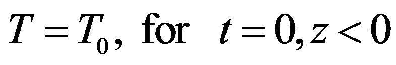
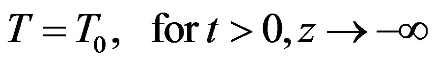
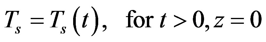
For a semi-infinite solid, bounded by a surface (z = 0) with extension to infinity in depth z, given a uniform initial temperature (T0) profile throughout the entire soil layer, the heat transfer process in the soil system can be described as
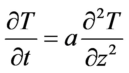 , (1a)
 , (1b)
 , (1c)
 , (1d)
where  is thermal diffusivity, T is soil temperature at depth z, and
  is surface soil temperature varying with time. We set
 , and Equations (1) is simplified to
 , (2a)
 , (2b)
 , (2c)
 . (2d)
This is a heat conduction problem with boundary temperature continuous in time. Such a problem can be solved with Duhamel’s theorem [25]. According to the theorem, if j(x, t) is the response of a linear system with a zero initial condition to a single, time-invariant non-homogeneous term with magnitude of unity (referred to as the fundamental solution), then the response of the same system,  , to a time-varying non-homogeneous term with magnitude B(t) can be obtained from the fundamental solution according to,
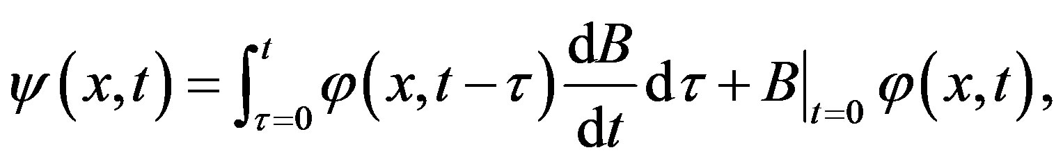 (3)
(3)
where  is the value of B at time zero and B must be continuous in time.
Likely, the solution of Equations (2) and (3) is given as
 (4)
(4)
where  is the integral variable, j(z, t) is the solution of the heat conduction problem with zero initial condition and a unity, time-invariant surface boundary temperature,
 , (5a)
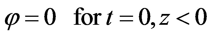 , (5b)
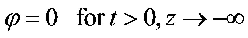 , (5c)
 (5d)
(5d)
Since j(z, t) is easy to solve using the separation of variables technique [26,27], we then have
 . (6)
. (6)
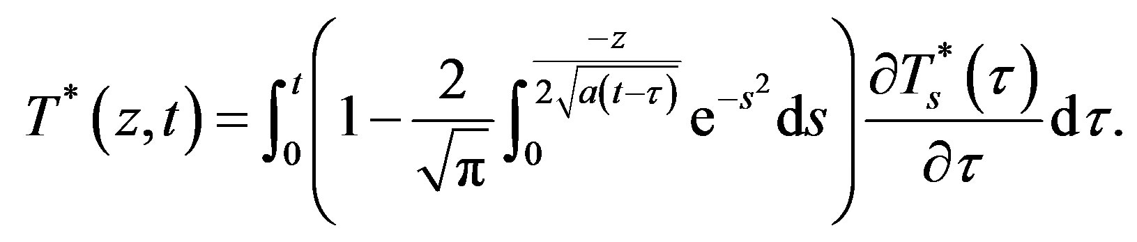
Substituting Equation (6) into Equation (4), we get
 (7)
(7)
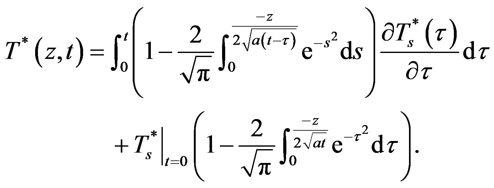
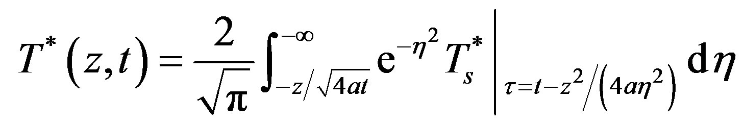
With the initial surface temperature  , we can obtain
 (8)
(8)
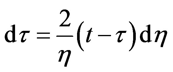
Resetting variable , subsequently we have
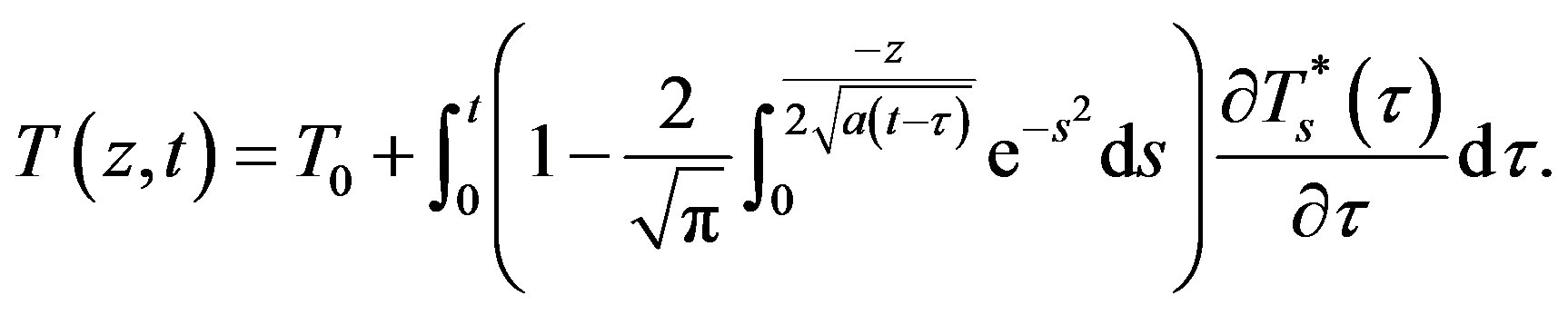 (9)
(9)
According to the Fourier’s law, soil heat flux (G) is proportional to the gradient of soil temperature (T), taking downward heat transfer as positive,
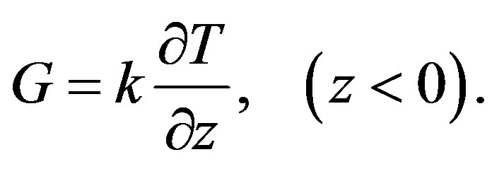 (10)
(10)
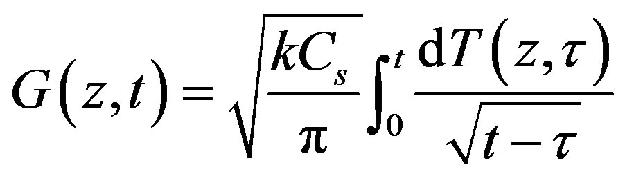
Combining Equations (9) and (10), we then get vertical soil heat flux
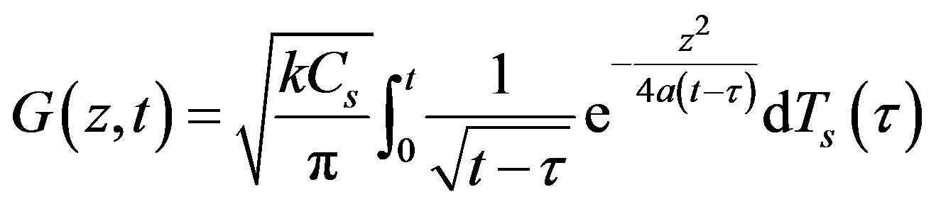 , (11)
where  is surface soil temperature, t is the integration variable, k is the heat conductivity (J∙m−1∙s−1∙K−1), and Cs is the volumetric heat capacity of soil
 . With Equation (11), we can estimate soil heat flux at any depth only from time series data of surface temperature when soil thermal properties are known.
In the following analysis, we make inferences to establish the linkages of Equation (11) to the existing singe-layer approaches. One is by Wang and Bras [18] (hereafter referred to as W-B approach), and another is by Horton and Wierenga [5] (hereafter referred to as H-W approach).
If the soil at depth  is set to be the upper boundary of the soil system, ceteris paribus, Equation (11) is expanded as
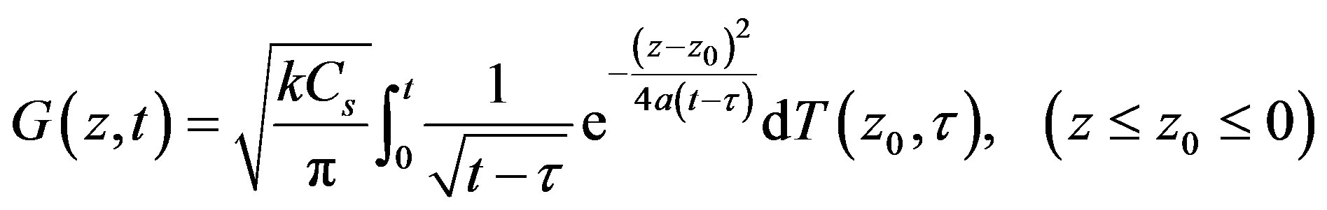 (12)
(12)
where  is soil heat flux at a deep layer below
 , and
, and  is soil temperature at
 . This means that the soil heat flux below can be obtained from time series of soil temperature at a certain depth. Inferentially, from Equation (12) soil heat flux at depth z is expressed as the integration of soil temperature at the same depth
 . (13)
Equation (13) is identical to that in the W-B approach, which was deduced with a half-order derivative/integral operator [18].
In the H-W approach, surface temperature is assumed as
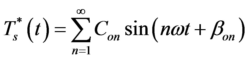 , (14)
where  is the amplitude of the nth harmonic of surface temperature, and
  is the nth phase constant. From Equation (8), we may have
 . (15)
If we define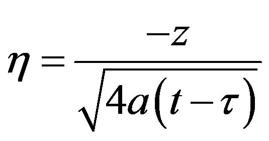 ,
,  , then Equation (15) becomes
 . (16)
Substituting Equation (14) into Equation (16), resetting variable , we may get
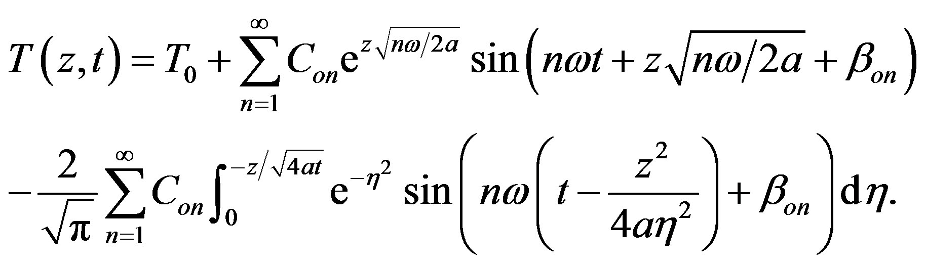 (17)
(17)
Likely, from Equation (10) we get
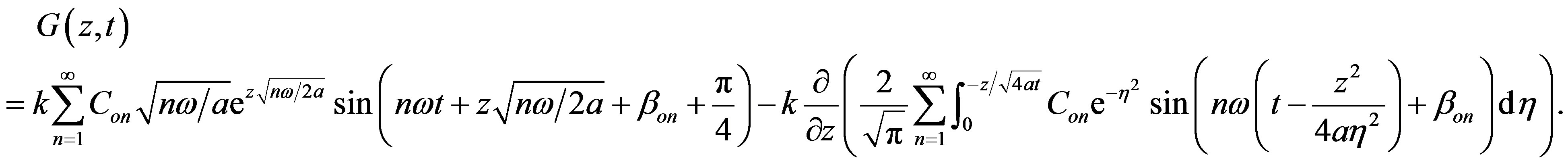 (18)
(18)
The second terms in (17) and (18) are transient processes. When time , they approach zero, leaving the first term which is a series with steady oscillation of periods
 [27]. In this case, Equation (18) becomes
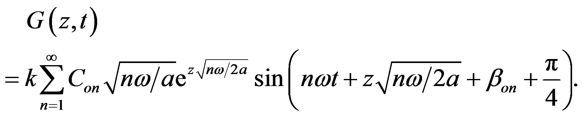 (19)
(19)
This is identical to the equation used in the H-W approach [5].
It is clear that Equation (13) is a derivative form of Equations (11) and (19) can be derived from Equation (9). In general, Equations (13) and (19) are derivatives of Equation (11). In this way, the generalized approach is linked to the W-B and the H-W approaches.
2.2. Error Propagation of Temperature Measure in the Generalized Approach
In regard to error propagation in Equation (11), if a Ts measure is supposed to be with both systematic and random errors, it can be described as follows
 , (20)
where ΔTs denotes systematic error (K) and δTs is random error (K). ΔTs may be constant or variable. Given that surface measures has a relative accuracy of A (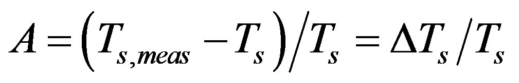 and |A| ≤ 1% in most cases), we may have
 . (21)
Further incorporated with Equation (11), we have
 .(22)
.(22)
Since the last component in Equation (22) is an improper integral, we get
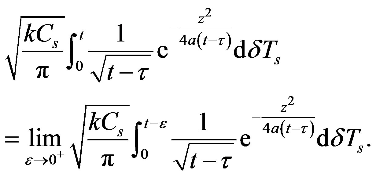 (23)
(23)
Based on the First mean value theorem for integration, there exists a value  such that
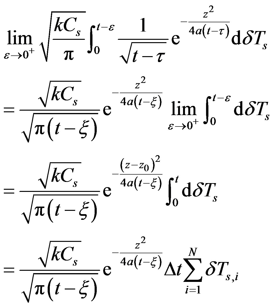 (24)
(24)
where Δt is time interval of Ts measures, N is the total number of measurements. From Equations (22)-(24), we get
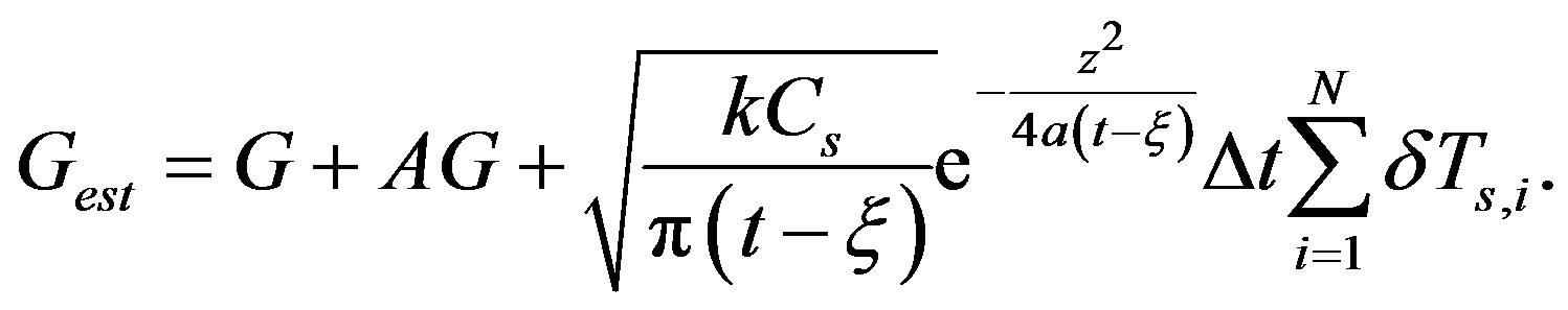 (25)
(25)
It is clear that Gest is affected by a systematic component AG and a random component
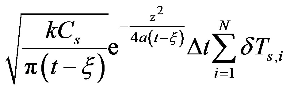 . Because
  is random error, its mathematical expectation
 . When N is large enough, the random component approaches zero. Providing that temperature measure has a relative error of 1% (approximate 3 K), it would result in 1% error in Gest. Therefore, it is expected that errors in surface temperature measure would have limited effects on the estimated soil heat flux.
3. Validation
Both model simulation and field observation were used for validation to test the generalized approach. Soil heat flux estimated from Equation (11) was compared with that simulated using heat transfer equation (Equations (1)) and heat flux equation (Equation (10)). Furthermore, the generalized approach was compared with the W-B approach and the H-W approach using field measures at two contrasting climate regimes.
3.1. Numerical Simulation
As did in Wang and Bras [18], numerical model of Equations (1) and (10) was established to test the generalized approach. To be representative for common soil materials, the coefficients, a used in Equation (1) and k and Cs used in Equations (10) and (11), were set to be 7.2 × 10⁻⁷ m2∙s−1, 1.0 W∙m−1∙K−1, and 1.4 × 10⁶ J∙m−3∙K−1, respectively. Given a function of Ts, surface soil heat fluxes can be subsequently calculated at a depth, for example, 5-cm. Meanwhile, Equation (11) was applied to estimate soil heat flux at the corresponding depth.
3.2. Case Examination
We used field data measured at two observation stations. Both sites are in China. The Shouxian site (32.55˚N, 116.78˚E) is in a humid monsoonal climate, and the Changwu site (35.2˚N, 107.8˚E) in a semi-arid climate. At Changwu, soil temperatures were measured at 2, 10, 20, and 40 cm depths, and soil heat flux was measured at 5 cm depth. At Shouxian, soil temperatures were observed at 5, 10, 20, and 40 cm, and soil heat flux was measured at 1 cm. Surface soil temperatures were measured with an infrared thermometer installed on a flux tower at each site [28,29]. The infrared thermometers were calibrated with an accuracy of ±2 K (one Standard Deviation), roughly 0.7% in relative accuracy. All the data were 30-min mean values. In this study, two-week observation data were selected at each site for the period when soil heat flux had large variations. This is, from 10-24 August 2003 at Shouxian, and from 15-29 July 2004 at Changwu.
The generalized approach, the W-B approach and the H-W approach were respectively used to estimate soil heat flux at 1 cm depth for Shouxian and at 5 cm depth for Changwu. The coefficient kCs used in Equations (11) and (13) was estimated following Wang and Bras [18]. The thermal diffusivity a used in Equations (11), (13) and (19) was estimated from soil temperature measurements using the arctangent approach [30].
The generalized approach (Equation (11)) requires only surface temperature. On the other hand, the W-B approach (Equation (13)) requires soil temperature data at the depth same as that of soil heat flux. Since the data were unavailable, cubic-spline interpolation approach was used to obtain soil temperature at the depth where soil heat flux was measured [1,31]. At Shouxian, T1cm was interpolated from the temperature data measured at 0, 5, 10, 20, and 40 cm depths. At Changwu, T5cm was interpolated from the temperature at 0, 2, 10, 20, and 40 cm depths. Following Wang and Bras [18] and Hsieh et al. [22], we set the initial values of a soil temperature profile to be uniform and the starting time of integration in Equations (11) and (13) to be the time when soil heat flux was close to zero.
The H-W approach requires a harmonics number and several coefficients used in Equation (19). To achieve satisfied results, the harmonics number was set to be 6 [32], and the coefficients  and
and  were used, not for the whole observation period, but for every 24-hour period in this study. Fourier series analysis was applied to surface temperature data in order to obtain the coefficients [17].
4. Results and Discussion
4.1. Validation of the Generalized Approach
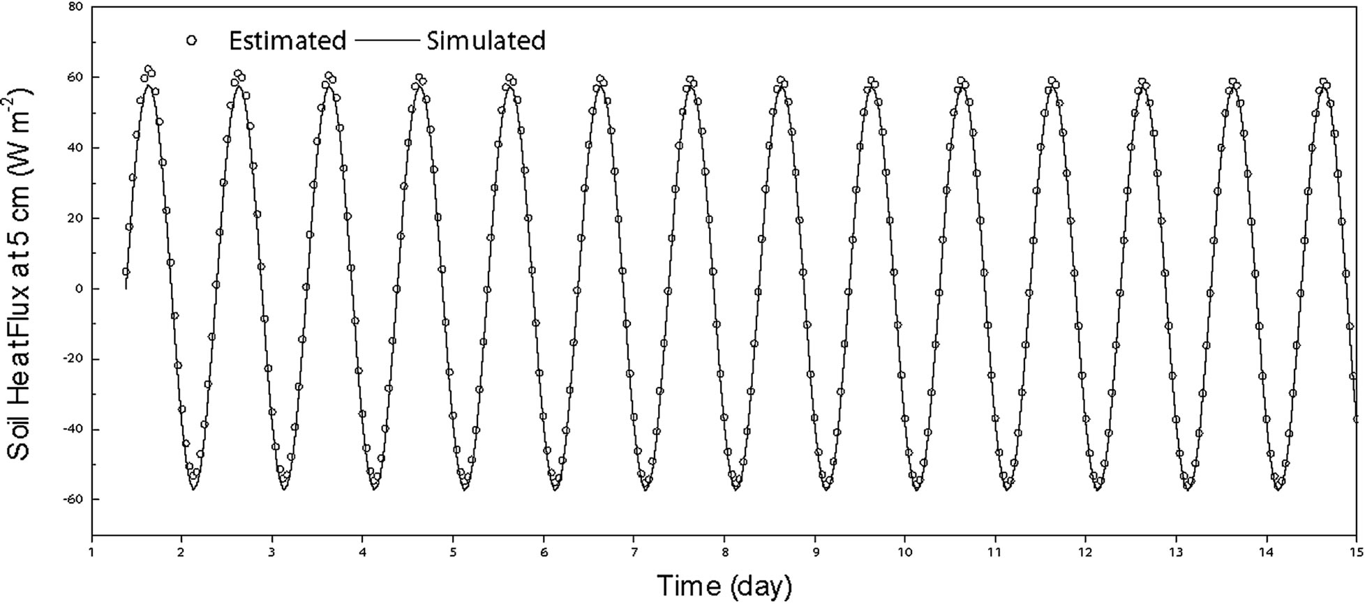
Results demonstrated that surface soil heat fluxes estimated from Equation (11) agreed well with that simulated from the heat transfer model (Figure 1(a)). The estimated and the model simulated fluxes had a high coefficient of R2 = 0.99 (p < 0.001) (Figure 1(b)), with a difference of 2.2 ± 0.8 W∙m−2 (one S. D.) and a Root Mean Square Error (RMSE) of 2.3 W∙m−2. It confirmed that the generalized approach is comparable to the numerical solution of the heat transfer equation.
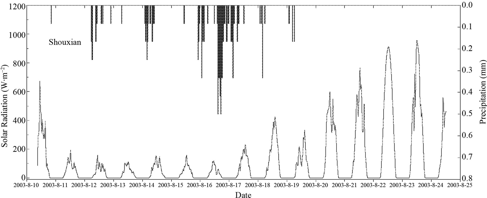
Figure 2 illustrates the environmental variations in terms of precipitation and solar radiation at Shouxian (Figure 2(a)) and Changwu (Figure 2(b)). At the Shouxian site, solar radiation was generally lower than 200 W∙m−2 during rainy periods and reached over 800 W∙m−2 in the later sunny days. At Changwu site, it was generally sunny and solar radiation reached over 1200 W∙m−2 in this period.
Figure 3 shows the temporal variations of soil temperature by depth at Shouxian (Figure 3(a)) and Changwu (Figure 3(b)). The average soil temperature was generally higher than 25˚C at Shouxian. Soil temperature showed the larger variation at Changwu than at Shouxian.
Figure 4 shows the temporal variations of soil heat flux (black line) observed by heat-flux plate at 1-cm depth for Shouxian (Figure 4(a)) and 5-cm depth for Changwu (Figure 4(b)). The overall average soil heat fluxes were −2.6 W∙m−2 and 1.3 W∙m−2 at the two sites during the observation periods. The overall average diurnal amplitudes were 44.5 W∙m−2 and 122.9 W∙m−2, respectively. In daytime, the soil heat flux was generally higher at the Changwu site than at the Shouxian site.
The soil heat flux estimates from Equation (11) (blue dot) basically agreed well with the observed values at both sites (Figure 4). At Shouxian, the estimated values from Equation (11) agreed with the observed values (R2 = 0.92) (p < 0.001) (Figure 5(a)), with a difference of 0.17 ± 4.9 W∙m−2 (Table 1). The RMSE was 4.9 W∙m−2. At Changwu, the estimates from Equation (11) agreed with the observed values (R2 = 0.89) (p < 0.001) (Figure 6(a)), showing a difference of 0.0 ± 13.4 W∙m−2, with a RMSE of 13.3 W∙m−2 (Table 1). Clearly, Equation (11) showed comparable performance in estimating soil heat flux at both Shouxian with a humid monsoonal climate and Changwu with a semi-arid climate.
4.2. Comparative Analysis of Three Approaches
The estimates of soil heat fluxes from the proposed, the W-B, and the H-W approaches are shown in Figure 4. The values from the proposed method Equation (11) were indicted with blue dot. The values from the W-B
 (a)
(a) (b)
(b)
Figure 1. Comparison of soil heat flux simulated from the heat transfer model and that estimated from the proposed equation (Equation (11)). (a) Time series of the model simulated and the estimated soil heat fluxes; (b) The model simulated versus the estimated soil heat flux.
approach were in red line and from the H-W approach in olive-line forms. The temporal variations of the observed and estimated soil heat flux are the evidence that all the three approaches agreed with the observation. The scatter plots of the estimated against the observed values confirmed the agreements (Figures 5 and 6). The values were distributed around 1:1 line. The slopes of regression lines were quite close to unity.
Among the three approaches, the proposed method showed best performance for both sites. The regression equations between the estimated values by Equation (11) and the measured values were  for Shouxian and
 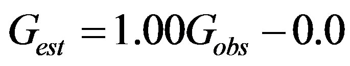 for Changwu. It had the highest correlation coefficient R2 and the lowest mean, S.D. and RMSE among the three approaches for both sites (Table 1).
The W-B approach performed well at Shouxian site (Figure 5(b)) but was less effective at Changwu. At Shouxian site, it had a difference to the observed values by 0.39 ± 5.1 W∙m−2. The R2 value was 0.92 (p < 0.001) and the RMSE was 5.2 W∙m−2, very close to that by the generalized approach. At Changwu site, the difference
 (a)
(a)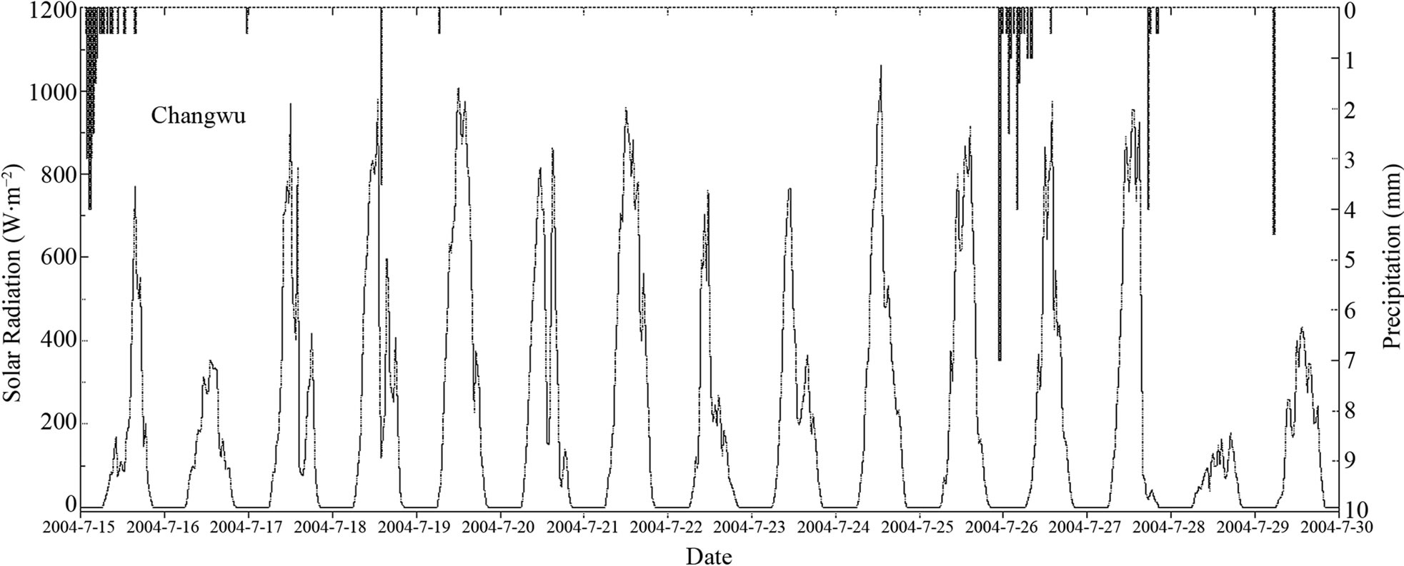 (b)
(b)
Figure 2. Environmental variations in terms of solar radiation and precipitation during the observation period at Shouxian (a) and Changwu (b) of China.
was −3.33 ± 27.5 W∙m−2. The R2 value was low by 0.67 (p < 0.05), and the RMSE value was 27.7 W∙m−2, more than two times of that by the generalized approach.
The H-W approach did not perform as well as that by the W-B approach at Shouxian. It had a difference to the observed values by 1.80 ± 14.2 W∙m−2. The R2 value between the estimates and the measures was 0.57 and the RMSE was 14.6 W∙m−2. On the other hand, it achieved good performance at Changwu with a difference of -1.3 ± 18.5 W∙m−2, a R2 of 0.83 (p < 0.01) and a RMSE of 18.7 W∙m−2. It showed better performance than the W-B approach at Changwu.
4.3. Evaluation of Three Approaches
From section 2.1, it is clear that the W-B approach and the H-W approach are derivative forms of the generalized approach. However, comparative analysis revealed the approaches showed different performance in estimating soil heat fluxes at either testing sites. In the section, we will make further analysis to investigate what should account for the differences in estimation.
The generalized approach achieved a high agreement with the observed soil heat flux. The errors in the estimation can be related to the measurement errors in land surface temperature and soil heat flux, the estimation of the coefficients representing soil thermal properties, and the assumptions used in derivation of the generalized approach as well. In the derivation of Equation (11), we assumed soil to be homogeneous and no internal heat sources exist. Homogeneity assumption requires soil ther-
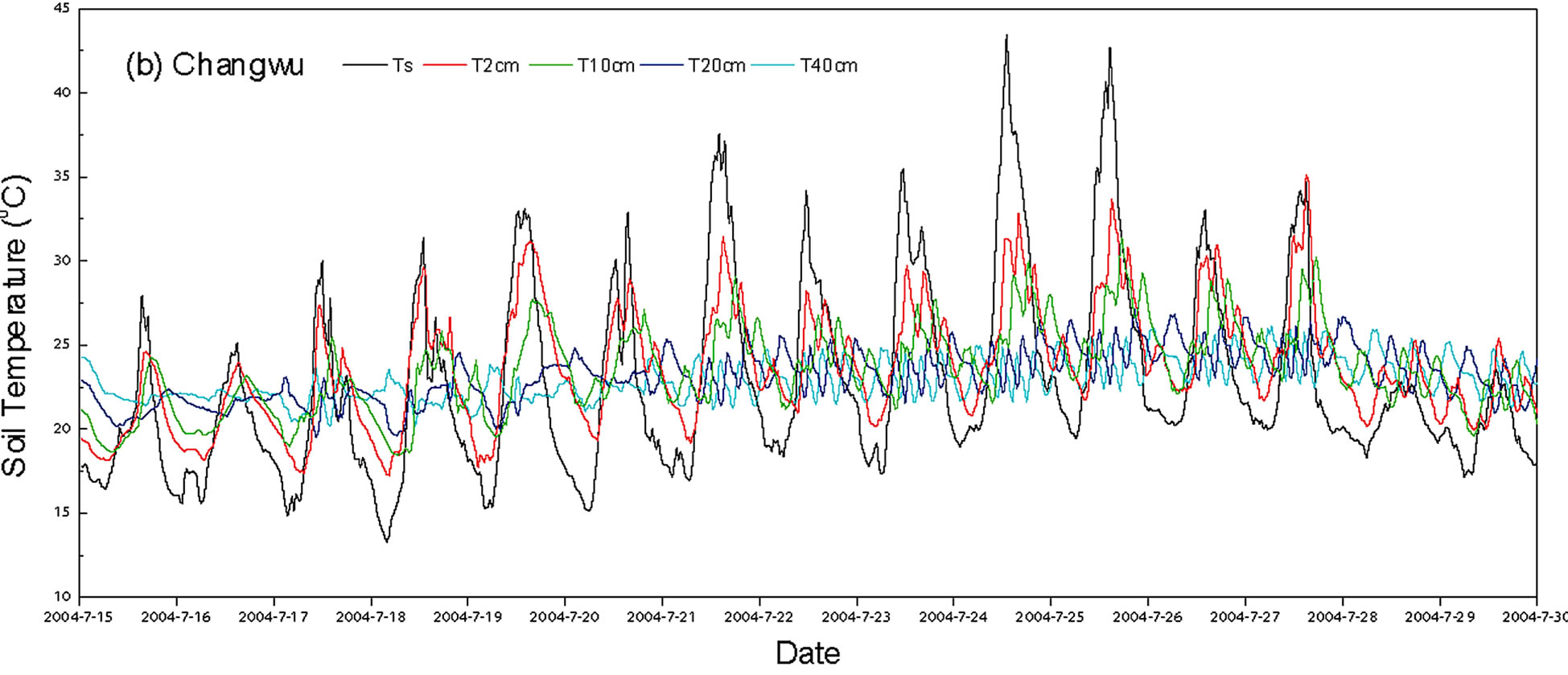
Figure 3. Temporal variations of soil temperatures by depth at Shouxian (a) and Changwu (b) of China during the observation periods.
mal properties, including heat conductivity k, heat capacity Cs and/or thermal diffusivity a, be invariant in space and time. In the present study, we used the same values for all the approaches. Our results showed that the estimated k, Cs and a values were relatively constant for different layers at Changwu or Shouxian. Consequently, the differences between different approaches were unlikely related to the homogeneity assumption and estimation errors in the coefficients.
The W-B approach achieved comparable results to the generalized approach at Shouxian site, but less comparable results by a difference of −0.69 ± 14.1 W∙m−2 at Changwu site. The difference between the generalized approach and the W-B approach was that the later required soil temperature to be measured at the same depth as that of the estimated soil heat flux. This is generally unavailable at a large scale, and its application is thus limited to cases when estimating soil heat flux on surface. In the present study, soil temperature data were unavailable at the same depth as the soil heat flux measurement at either Shouxian or Changwu. Thus, the cubic-spline interpolation approach was used to obtain the required soil temperature. The statistically-based approach may generate errors in the interpolated temperature. For example, in the case of Shouxian, the vertical distribution of soil temperature was relatively stable within a relatively narrow range of temperature during the observation period. Figure 7(a) shows a one-day case. In the case of Changwu, surface soil temperature had a relatively large variation within a relatively wide range of temperature. The large fluctuations tended to increase the errors in the interpolated temperature compared to that at Shouxian (Fig-
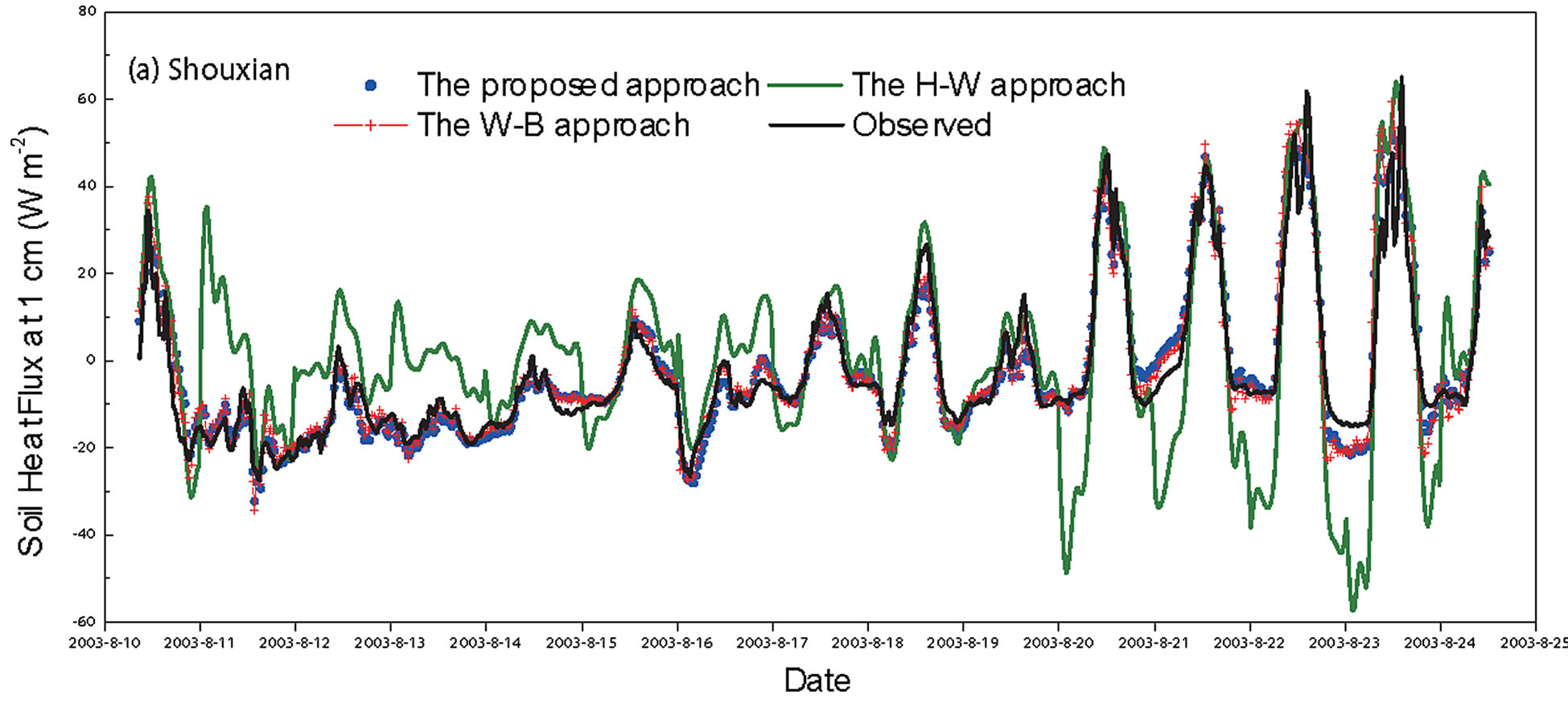
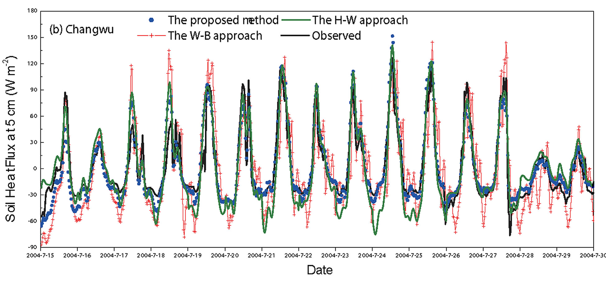
Figure 4. Temporal variations of soil heat fluxes observed (black line) and estimated from the generalized approach (blue dot), the W-B approach (red line) and the H-W approach (olive line) at a depth of 1-cm at Shouxian (a) and 5-cm at Changwu (b) of China during the observation period.
ure 7(b)). The interpolation errors were responsible for the resulted errors in soil heat flux, especially at Changwu.
Compared the generalized approach, the H-W approach did not achieve satisfactory results at Shouxian as it did at Changwu. Its difference to the generalized approach was that it assumed soil temperature and soil heat flux varied harmonically with time. This hypothesis is not always fulfilled, particularly in regions where abrupt weather change occurs within a short time, for example, during the crossover of a cold front [33]. Furthermore, the H-W approach requires determination of harmonics number. Although it was declared that any periodic variation could be well simulated if the number was large enough, in practice only limited number can be used and this would inevitably introduce errors, sometimes quite large, in estimation. In the present study, we used six harmonics, which was quite high to estimate soil heat flux for every 24-hour period. In addition, the coefficients in Equation (19) need to be estimated using the Fourier series analysis. The errors in the coefficients can also result in the errors in the estimation. Overall, the combined effects may produce large errors in estimated soil heat flux. An indirect evidence was that there existed a difference between the interpolated temperature and the temperature using the harmonic expression (Equation (14)) by −0.2 ±

Figure 5. Comparison of observed soil heat flux against estimated values from the generalized approach (a), the W-B approach (b), and the H-W approach (c) at a depth of 1-cm at Shouxian of China.
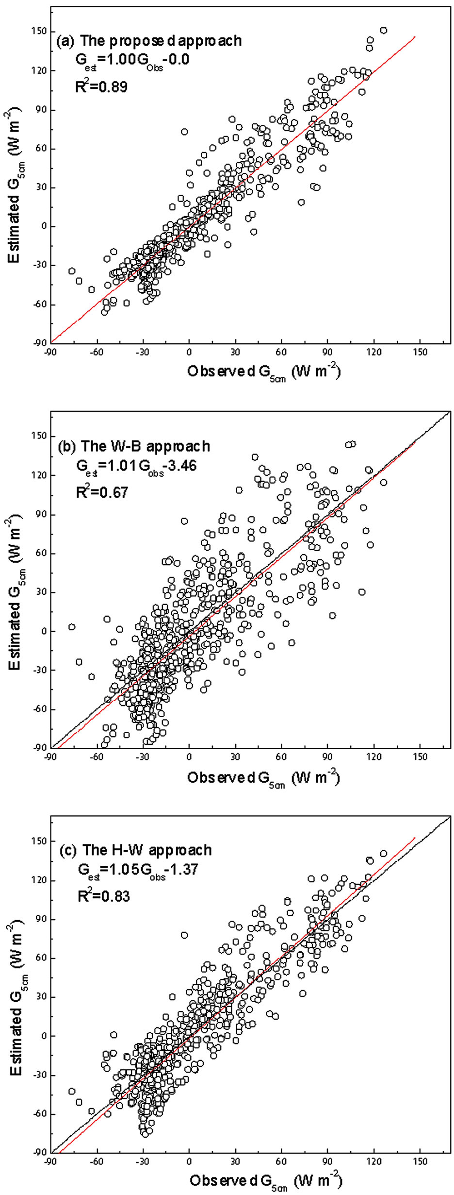
Figure 6. Comparison of observed soil heat flux against estimated values from the generalized approach (a), the W-B approach (b), and the H-W approach (c) at a depth of 5-cm at Changwu of China.
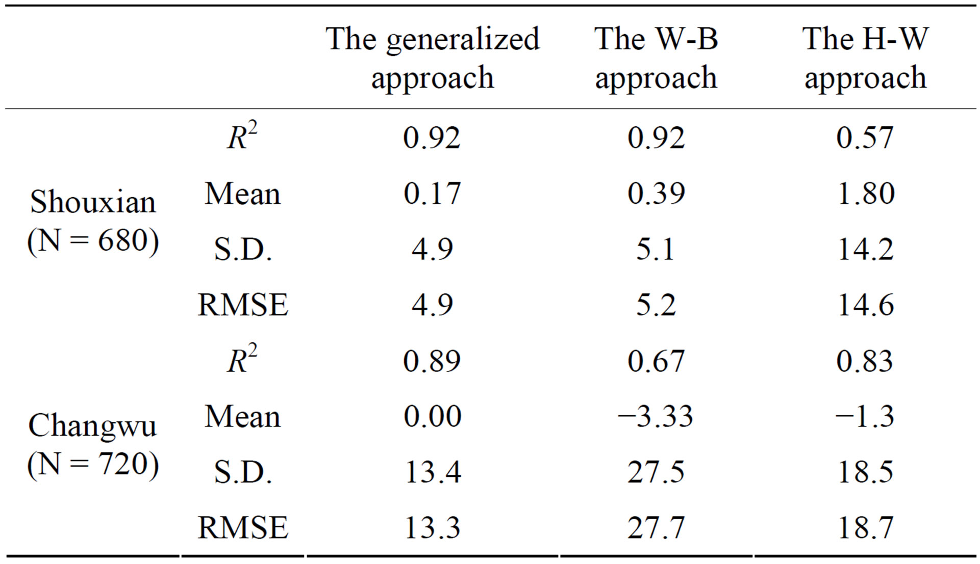
Table 1. Statistical differences between the observed soil heat flux against the estimated values from the generalized approach, the W-B approach and the H-W approach at Shouxian and Changwu of China.
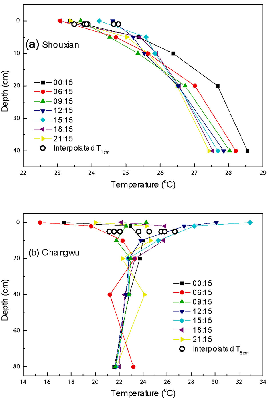
Figure 7. Diurnal variation in profile of soil temperature at Shouxian (a) and Changwu (b) of China. The circles indicated the temperature calculated by the cubic-spline interpolation approach.
0.7˚C on average at a depth of 1 cm at Shouxian. The difference generated the discrepancy between the soil heat fluxes estimated from the W-B approach and the H-W approach by −3.0 ± 13.4 W∙m−2. Figure 8 illustrated the statistical relationship between the tempera-
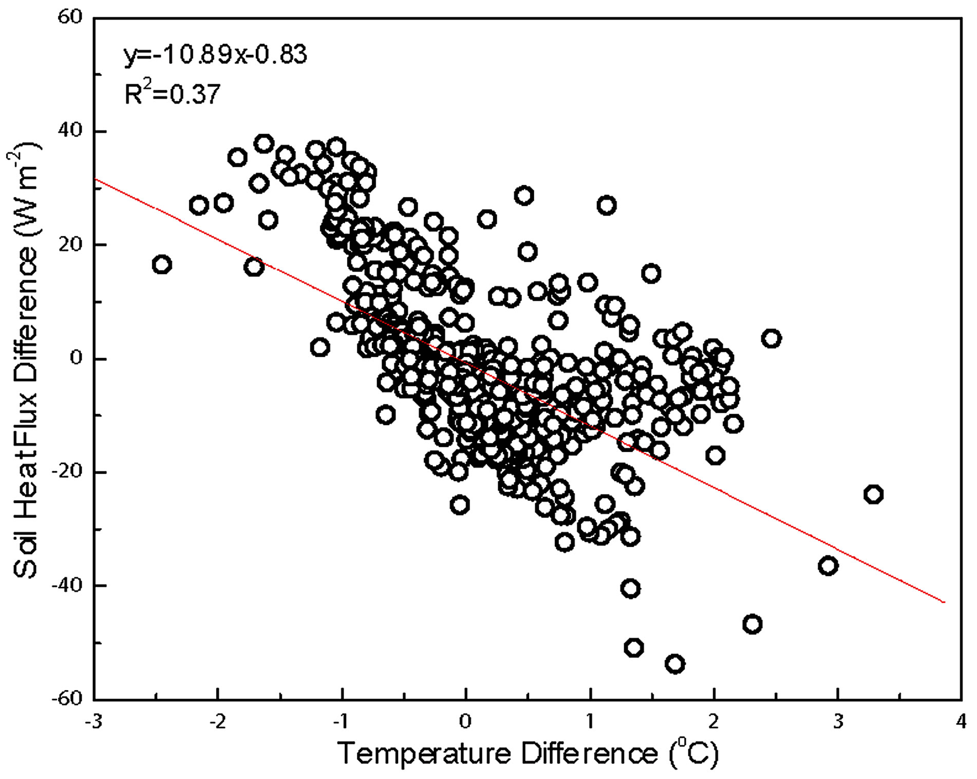
Figure 8. Statistical relationships between the temperature difference and the soil heat flux difference at a depth of 1-cm at Shouxian of China. The temperature difference refers to the difference between the values calculated from the cubic-spline interpolation approach and that from the harmonic equation (Equation (14)). The soil heat flux difference refers to the difference between the values estimated by the W-B approach and by the H-W approach.
ture difference and the soil heat flux discrepancy. One degree temperature difference could produce approximate 10 W∙m−2 at the site. Therefore, use of the cubicspline interpolation should be with caution to obtain inner soil temperature for the H-W approach.
In general, all these approaches can be used for estimating soil heat flux using single-layer data. The generalized approach is superior to the W-B approach and the H-W approach in that it has less restrictions and assumptions but higher overall accuracy. The approach can estimate soil heat flux at any depth but it requires only surface temperature data as input, which appears to be an advantage to remote sensing applications. Even errors in temperature measure make limited effects on soil heat flux estimates, yet it faces difficulty when applied to satellite remote sensing. One of the difficulties is that it is difficult for remote sensing to accurately estimate K, Cs, or a. While the present study is validated at in situ scale, further extensive investigation is necessary for expanding its application to large scale.
5. Conclusions
The Duhamel’s theorem was used to derive Equation (11) for estimating soil heat flux at any depth solely from time series of surface temperature measurements. This equation can be extended to estimate soil heat flux below a given depth if soil temperature at that depth is known. The W-B approach is a derivative form of the generalized approach. With temperature expressed with harmonic equation, we also derived the H-W approach from the generalized approach. Of all these approaches, the generalized approach offers a way with less restriction and assumptions to estimate soil heat flux.
Error analysis revealed that measurement errors in surface temperature would have limited effects on soil heat flux estimates from the generalized approach. Model simulation showed that soil heat flux estimated from the generalized approach agreed quite well with the simulated from heat transfer equation. Furthermore, case examinations demonstrated that it achieved best performance at two observation sites with contrasting climate regimes. The W-B approach achieved better results at Shouxian, and the H-W approach did better at Changwu. The error sources were related to the assumptions and estimation errors in the coefficients used in each approach. In general, Equation (11) was recommended for practical use in estimating soil heat flux. Further investigation is necessary if the approach is applied at a large scale.
Acknowledgements
This work was jointly supported by a Key Program of Nanjing Institute of Geography and Limnology, Chinese Academy of Sciences (CAS) (NIGLAS2012135001) and the CAS 100-talent Project. We thank Dr H Tanaka for his kind assistance in data acquiration and his valuable comments to improve the early manuscript.
REFERENCES
- J. Ogée, E. Lamaud, Y. Brunet, P. Berbigier and J. M. Bonnefond, “A Long-Term Study of Soil Heat Flux under a Forest Canopy,” Agricultural and Forest Meteorology, Vol. 106, No. 3, 2001, pp. 173-186. http://dx.doi.org/10.1016/S0168-1923(00)00214-8
- B. A. Kimball, R. D. Jackson, F. S. Nakayama, S. B. Idso and R. J. Reginato, “Soil-Heat Flux Determination: Temperature Gradient Method with Computed Thermal Conductivities,” Soil Science Society of America Journal, Vol. 40, No. 1, 1976, pp. 25-28. http://dx.doi.org/10.2136/sssaj1976.03615995004000010011x
- T. R. Oke, “Boundary-Layer Climates,” Methuen, New York, 1987.
- C. L. Mayocchi and K. L. Bristow, “Soil Surface Heat Flux: Some General Questions and Comments on Measurements,” Agricultural and Forest Meteorology, Vol. 75, No. 1-3, 1995, pp. 43-50. http://dx.doi.org/10.1016/0168-1923(94)02198-S
- R. Horton and P. J. Wierenga, “Estimating the Soil Heat Flux from Observation of Soil Temperature near the Surface,” Soil Science Society of America Journal, Vol. 47, No. 1, 1983, pp. 14-20. http://dx.doi.org/10.2136/sssaj1983.03615995004700010003x
- C. Liebethal and T. Foken, “Evaluation of Six Parameterization Approaches for the Ground Heat Flux,” Theoretical and Applied Climatology, Vol. 88, No. 1-2, 2007, pp. 43-56. http://dx.doi.org/10.1007/s00704-005-0234-0
- C. B. Tanner, “Basic Instrumentation and Measurement for Plant Environment and Micrometeorology,” Univ. of Wisconsin Madison Soils Bull. No. 6, 1963.
- J. P. Pandolfo, D. S. Cooley and M. A. Atwater, “The Development of a Numerical Prediction Model for the Planetary Boundary Layer,” Final Report, the Travelers Research Center, Inc., Hartford, 1965, 88 p.
- M. Tang, W. Dong, B. Wang and J. Zhang, “The Heat Flow Field of Soil and the Comparison between It and That Deep-Layer in China,” Advanced Earth Sciences, Vol. 6, No. 4, 1991, pp. 10-17.
- B. S. Sharratt, G. S. Campbell and D. M. Glenn, “Soil Heat Flux Estimation Based on the Finite-Difference form of the Transient Heat Flow Equation. Agricultural and Forest Meteorology, Vol. 61, 1992, pp. 95-111. http://dx.doi.org/10.1016/0168-1923(92)90027-2
- C. Li, T. Duan, L. Chen, W. Li, J. Shuo, S. Hagonoya and T. Satou, “Calculation of the Soil Heat Exchange in Qinghal-Tibet Plateau,” Chengdu Institute of Plateau Meteorology, Vol. 14, No. 2, 1999, pp. 129-138.
- K. Tanaka, H. Ishikawa, T. Hayashi, I. Tamagawa and Y. Ma, “Surface Energy Budget at Amdo on the Tibetan Plateau Using GAME/Tibet IOP98 Data,” Meteorological Society of Japan, Vol. 79, No. 1B, 2001, pp. 505-517. http://dx.doi.org/10.2151/jmsj.79.505
- K. Yang and J. Wang, “A Temperature Prediction-Correction Method for Estimating Surface Soil Heat Flux from Soil Temperature and Moisture Data,” Science in China Series D: Earth Science, Vol. 51, No. 5, 2008, pp. 721-729. http://dx.doi.org/10.1007/s11430-008-0036-1
- D. Weng, Q. Gao and F. He, “Climatologcal Calculations and Distribution of Soil Heat Flux over China,” Scientia Meteorological Sinica, Vol. 14, No. 2, 1994, pp. 91-97.
- Y. Ma, Z. Su, Z. Li, T. Koike and M. Menenti, “Determination of Regional Net Radiation and Soil Heat Flux Densities over Heterogeneous Landscape of the Tibetan Plateau,” Hydrological Processes, Vol. 16, No. 15, 2002, pp. 2963-2971. http://dx.doi.org/10.1002/hyp.1079
- W. Van Wijk and D. de Vries, “Periodic Temperature Variations in a Homogeneous Soil,” In: W. R. Van Wijk, Eds., Physics of Plant Environment, North-Holland Publ. Co., Amsterdam, 1963, pp. 102-143.
- A. Verhoef, “Remote Estimation of Thermal Inertia and Soil Heat Flux for Bare Soil,” Agricultural and Forest Meteorology, Vol. 123, No. 3-4, 2004, pp. 221-236. http://dx.doi.org/10.1016/j.agrformet.2003.11.005
- J. Wang and R. L. Bras, “Ground Heat Flux Estimated from Surface Soil Temperature,” Journal of Hydrology, Vol. 216, No. 3-4, 1999, pp. 214-226. http://dx.doi.org/10.1016/S0022-1694(99)00008-6
- H. Beltrami, “Surface Heat Flux Histories from Inversion of Geothermal Data: Energy Balance at the Earth’s Surface,” Journal of Geophysical Research: Solid Earth, Vol. 106, No. B10, 2001, pp. 21979-21993. http://dx.doi.org/10.1029/2000JB000065
- H. Beltrami, J. Wang and R. Bras, “Energy Balance at the Earth’s Surface: Heat Flux History in Eastern Canada,” Geophysical Research Letters, Vol. 27, No. 20, 2000, pp. 3385-3388. http://dx.doi.org/10.1029/2000GL008483
- T. R. H. Holmes, M. Owe, R. A. M. De Jeu and H. Kooi, “Estimating the Soil Temperature Profile from a Single Depth Observation: A Simple Empirical Heatflow Solution,” Water Resources Research, Vol. 44, No. 2, 2008, Article ID: WO2412. http://dx.doi.org/10.1029/2007WR005994
- C. Hsieh, C. Huang and G. Kiely, “Long-Term Estimation of Soil Heat Flux by Single Layer Soil Temperature,” International Journal of Biometeorology, Vol. 53, No. 2, 2009, pp. 113-123. http://dx.doi.org/10.1007/s00484-008-0198-8
- Z. Wan and Z. Li, “A Physics-Based Algorithm for Retrieving Land-Surface Emissivity and Temperature from EOS/MODIS Data,” IEEE Transactions on Geoscience and Remote Sensing, Vol. 35, No. 4, 1997, pp. 980-996. http://dx.doi.org/10.1109/36.602541
- O. C. Justice, E. Vermote, J. R. G. Townshend, R. Defries, D. P. Roy, D. K. Hall, V. V. Salomonson, J. L. Privette, G. Riggs, A. Strahler, W. Lucht, R. B. Myneni, Y. K. Knyazikhin, S. W. Running, R. R. Nemani, Z. Wan, A. R. Huete, W. V. Leeuwen, R. E. Wolfe, L. Giglio, J. Muller, P. Lewis and M. J. Barnsley, “The Moderate Resolution Imaging Spectroradiometer (MODIS): Land Remote Sensing for Global Change Research,” IEEE Transactions on Geoscience and Remote Sensing, Vol. 36, No. 4, 1998, pp. 1228-1250. http://dx.doi.org/10.1109/36.701075
- L. A. Vegvilla-Berdecia, “Duhamel’s Theorem,” Journal of Chemical Education, Vol. 46, No. 5, 1969, pp. 312-314. http://dx.doi.org/10.1021/ed046p312
- M. N. Ozisik, “Heat Conduction,” John Wiley & Sons Inc., New York, 1980.
- H. S. Carslaw and J. C. Jaeger, “Conduction of Heat in Solids,” Clarendon Press, Oxford, 1986.
- T. Hiyama, A. Takahashi, A. Higuchi, M. Nishikawa, W. Li and Y. Fukushima, “Atmospheric Boundary Layer (ABL) Observations on the ‘Changwu Agro-Ecological Experimental Station’ over the Loess Plateau, China,” AsiaFlux Newsletter, Vol. 16, 2005, pp. 5-9.
- H. Tanaka, T. Hiyama, K. Yamamoto, H. Fujinami, T. Shinoda, A. Higuchi, S. Endo, S. Ikeda, W. Li and K. Nakamura, “Surface Flux and Atmospheric Boundary Layer Observations from the LAPS Project over the Middle Stream of the Huaihe River Basin in China,” Hydrological Processes, Vol. 21, No. 15, 2007, pp. 1997-2008. http://dx.doi.org/10.1002/hyp.6706
- R. Horton, P. J. Wierenga and D. R. Nielsen, “Evaluation of Methods for Determining the Apparent Thermal Diffusivity of Soil near the Surface,” Soil Science Society of America Journal, Vol. 47, No. 1, 1983, pp. 25-32. http://dx.doi.org/10.2136/sssaj1983.03615995004700010005x
- W. H. Press, S. A. Teukolsky, W. T. Vetterling and B. P. Flannery, “Numerical Recipes in Fortran, the Art of Scientific Computing,” 2nd Edition, Cambridge University Press, Cambridge, 1992, 963 p.
- X. Mo, H. Li, S. Liu and Z. Lin, “Estimation of Soil Thermal Conductivity and Heat Flux in near Surface Layer from Soil Temperature,” Chinese Journal of Eco-Agriculture, Vol. 10, No. 1, 2002, pp. 62-65.
- A. M. B. Passerat de Silans, B. A. Monteny and J. P. Lhomme, “Apparent Soil Thermal Diffusivity, a Case Study: HAPEX-Sahel Experiment,” Agricultural and Forest Meteorology, Vol. 81, No. 3-4, 1996, pp. 201-216. http://dx.doi.org/10.1016/0168-1923(95)02323-2
NOTES
*Corresponding author.