Modern Economy
Vol. 4 No. 7 (2013) , Article ID: 34710 , 7 pages DOI:10.4236/me.2013.47052
A Late 20th Century European Climate Shift: Fingerprint of Regional Brightening?
1Royal Netherlands Meteorological Institute (KNMI), De Bilt, The Netherlands
2Amsterdam, The Netherlands
Email: *laatdej@knmi.nl
Copyright © 2013 A. T. J. de Laat, M. Crok. This is an open access article distributed under the Creative Commons Attribution License, which permits unrestricted use, distribution, and reproduction in any medium, provided the original work is properly cited.
Received April 21, 2013; revised May 20, 2013; accepted May 30, 2013
Keywords: Temperature; Climate Shift; Brightening
ABSTRACT
We investigate the spatial extent of a statistically highly significant shift in atmospheric temperatures over Europe around 1987-1988 using a boot-strap change point algorithm. According to this algorithm, this change point (average warming of about one degree Celsius) is statistically highly significant (p > 99.9999%). The change point is consistently present in satellite and surface temperature measurements as well as temperature re-analyses and ocean heat content over most of Western Europe. We also find a connection with parts of the North Atlantic Ocean and eastern Asia. Although the time of change coincides with the North Atlantic Oscillation (NAO) going from negative to positive, the consistent warmer temperatures throughout the decades after 1987-1988 do not coincide with a persistent shift of the NAO, as it returns to a neutral/negative in the 1990’s. Furthermore, the shift does not coincide with any other known mode of multidecadal internal climate variability. We argue that the notion of a shift is “spurious”, i.e. the result of a fast change in Europe from dimming to brightening combined with an accidental sequence of cold (negative NAO) and warm (positive) NAO years during this period. The “shift” could therefore be considered as a fingerprint of European brightening during the last few decades.
1. Introduction
In recent decades Western Europe has been warming significantly faster than the world as a whole [1]. No generally accepted explanation for this faster increase in temperatures has been reported, although a decrease in aerosols due to improved air quality as well as circulation changes have been suggested as possible explanations [1-6].
However, a case can be made that this warming has not occurred gradually but it’s rather abrupt in the late 1980’s. We denote this idea as the “European Climate Shift” or ECS. This shift has been reported for local measurements around the Baltic area [6-8], but its spatial extent has remained unexplored. To illustrate where this idea of an ECS stems from, we present the Central Netherlands Temperature (CNT) record [9]. This homogeneous time series from 1906 onwards is representative for temperatures of a larger area in and around the Netherlands and is specifically constructed to study large-scale temperature changes. The reconstruction accounts for various effects, including changes in measurement method, measurement location and urbanization.
Figure 1(a) shows the CNT temperature record since 1906. Clearly there has been an increase in annual mean temperatures from about 1980 onwards. The temperature trend since 1980 has been 0.42 ± 0.26 K/decade (2σ uncertainty), using an ordinary linear regression. The timing of the temperature increase is consistent with the observed global mean temperature increase, but the magnitude of the warming is much larger than the global mean temperature change over that period [1]. However, even by visual inspection a case could be made that the temperature increase since 1980 is not gradual, but is dominated by a temperature shift around 1987-1988. When calculating trends before and after 1987, we found that the temperature trend from 1906 to 1987 has been 0.04 ± 0.06 K/decade, whereas the trend after 1987 has been 0.15 ± 0.37 K/decade. The change in average temperature before and after 1987 is 1.11 K. When investigating the residual temperatures after removing the trends, there is no clear difference in statistical properties of the residuals and it thus cannot be decided based on this statistic which model is better: a linear trend or a shift plus a linear trend. Hence, the possibility of a climate shift around 1987-1988 remains.
Climate change is generally defined within the framework of statistics. IPCC [10] provides a useful definition of “climate change”: “a change in the state of the climate that can be identified (e.g., by using statistical tests) by changes in the mean and/or the variability of its properties and that persists for an extended period, typically decades or longer.” It is thus important to investigate the possibility of a shift by independent statistical means. In this study we use a well-established change point analy-
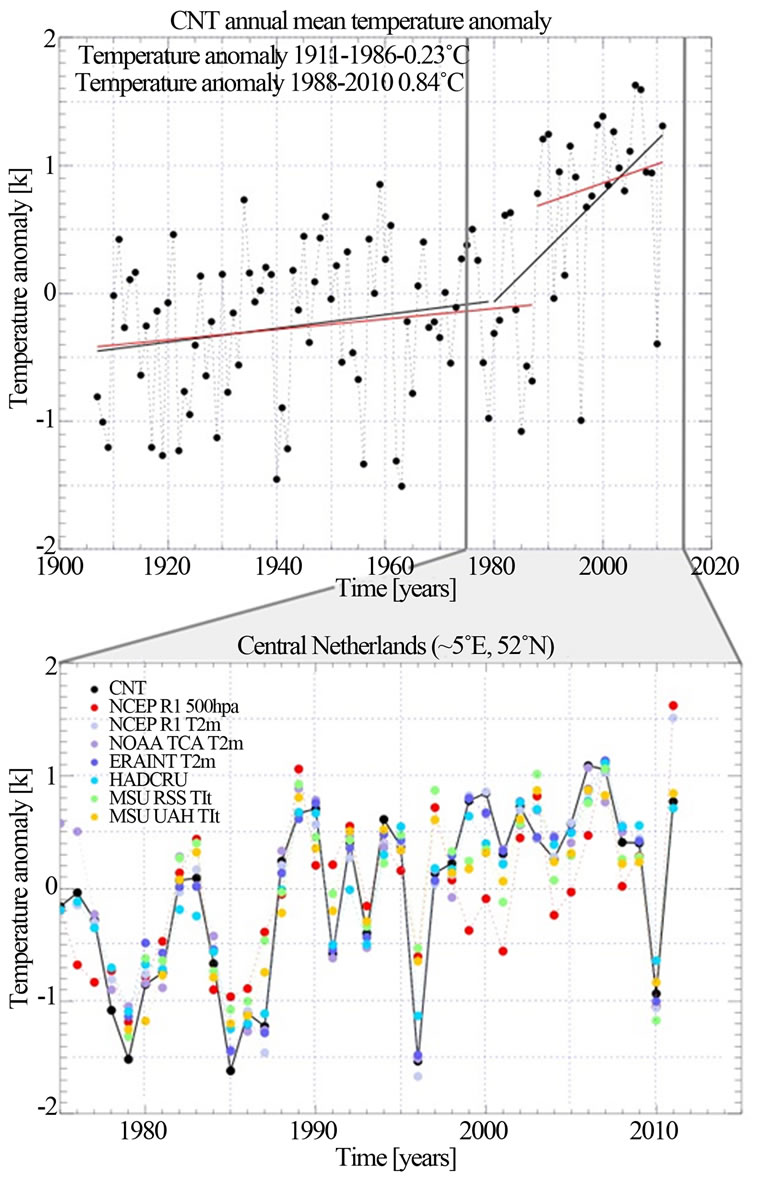
Figure 1. (a) Central Netherlands temperature anomaly with regard to the mean temperature from 1906-2011. The black line indicates the ordinary linear regressions before and after 1980, the red line indicates the same regression but before and after 1987. The colored points indicate periods of at least three consecutive years when temperatures for all years were smaller (blue) or larger (red) than half the root-mean-square value of temperature variability between 1906 and 1984. (b) Temperature anomalies with respect to the 1979-2010 mean for seven gridded temperature datasets for the Netherlands grid point for the period 1975-2011, as well as the Central Netherlands Temperature (black).
sis (CPA) algorithm for the identification of change points. The CPA algorithm used in this study also provides confidence intervals based on the bootstrap. We first subject the CNT record to the CPA algorithm to see if a shift can be identified. We then analyze temperature series over the Netherlands from other data sources using the same methodology for consistency. We extend the analysis to the European domain and end with an analysis of global patterns to investigate the geographical extent of the ECS, and end with a discussion of possible causes. For all analyses performed and datasets used, we use annual mean temperatures.
2. Methods and Data
2.1. Change-Point Analysis
For the detection of shifts in time series we use the change-point analysis (CPA) procedure [11,12]. The CPA algorithm is a non-parametric change point detection technique, which means that it does not presume certain statistical properties of the data to be analyzed. A bootstrap procedure is applied to estimate significance levels [13]. Change point analysis techniques are commonly used in climate research [14]. The basis of the CPA is the cumulative sum method (CUSUM). The cumulative sum is defined as:
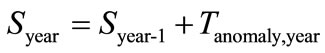
In which Syear denotes the cumulative sum for a given year and Tanomaly,year is the temperature anomaly for a given year with respect to the average of the entire temperature time series. By definition, the cumulative sum at time step zero (S0) is set at zero. The changes of cumulative sum can be used to determine changes by identifying points where the cumulative sum changes direction.
An important aspect of the identification of a change point is to determine their statistical significance. How can we be sure that a change did not occur by chance? Within the CPA method, statistical significance levels can be determined by using a bootstrap method. First, an estimator of the magnitude of the change is required. For this we use the difference between the minimum and maximum value of the cumulative sum (S).
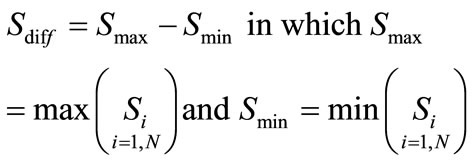
Smax and Smin are the maximum and minimum values of the cumulative sum during the period under consideration. We then generate a bootstrap sample of the length of the record by randomly reordering the original record (“sampling without replacement”). This bootstrapped series is then subjected to the CUSUM method again, providing a bootstrapped cumulative sum difference ( ). The idea is that “the bootstrap sample represents random re-orderings of the data as if no change has occurred”. By performing a large number of such bootstraps one gets an estimate of the range of Sdiff values as if no change would have occurred. With the large number of realizations a confidence interval can be defined, i.e. the number of bootstrapped
  values larger than the Sdiff represents the chance that the change may have occurred by chance. One particular advantage of a bootstrapping method is that measurement errors are implicitly taken into account: variations in a parameter related to measurement errors are included in the confidence estimates as the original data is continually resampled in the bootstrap method. A disadvantage of the bootstrap is that it is a computationally expensive method: the typical number of bootstraps that is required is 1000 for a given time series and this limitation to 1000 is because of practical reasons. Analyzing multiple datasets would otherwise consume too much time. For example, the calculation of the 5 million resamplings as reported in this study took more than one day of computation on a common desktop computer. The confidence intervals thus have their own uncertainties, but using 1000 bootstraps is a generally accepted procedure.
Once the CPA method has been applied to the time series, it is split at the change point into two separate time series. For both time series the CPA analysis is repeated again, and so forth until certain criteria are met. In this paper, the criteria we use are the following:
1) The confidence interval must be larger than 95% for positive change point detection.
In general it is assumed that a confidence interval smaller than 95% (two standard errors in case of a Gaussian distribution) indicates that the change cannot be considered different from having occurred by chance. This does not mean that any change with a confidence interval larger than 95% means that a change did occur, but it is a first filter.
2) Time series analyzed for change points contain at least 10 years of data.
The latter is motivated by the notion that we are interested in decadal changes in climate and temperatures (see the definition of climate change in the introduction). Climate variations on shorter time scales are thus filtered out.
2.2. Datasets
All datasets used in this study were obtained from the KNMI Climate Explorer database (http://climexp.knmi.nl). We use the Central Netherlands Temperature record, one of the best documented long term temperature records available [9]. We further use the lower tropospheric satellite temperature records from the Microwave Sounding Unit (MSU) satellites from both the University of Alabama/Huntsville (UAH, v5.4 [15]) and Remote Sensing Systems (RSS, v3.3 [16]), which is available from 1979 onwards. In addition, we also use the National Center for Environmental Protection (NCEP) R1 reanalysis [17] 500 hPa and 2-meter temperature data which starts in 1948. We further use European Center for Medium Weather Forecast interim reanalysis (ERA INTERIM [18]) which starts also in 1979. We also use the combined CRUTEM3 and HADSST2 surface temperature product available at the KNMI climate explorer, both from the Hadley Center in the United Kingdom [19-22], and we use the National Oceanic and Atmospheric Administration (NOAA) PSD Twentieth Century Analysis dataset [23-25]. These last two datasets are the longest available gridded datasets, going back to 1850 and 1870, respectively. For analysis purposes, we also include Ocean Heat Content (OHC) data from the National Oceanic Data Center [26], which starts in 1955. A summary of the characteristics of all datasets is given in Table 1.
3. The Central Netherlands Temperature
As outlined earlier, this research was motivated by the visual inspection of temperature records in the Netherlands, which showed warming after about 1980. For illustration purposes, the data was separated into two parts —before and after 1980 (black) or 1988 (red)—and fitted with an Ordinary Linear Regression (OLR). The mean temperature anomalies before and after 1987 are −0.23 and 0.84 K, respectively, resulting in a mean temperature difference of 1.1 K.
Although we could make a case that a shift occurs around 1987, from this visualization we can see that it is difficult to determine which model (linear + linear or linear + shift + linear) is better. The root-mean-square (RMS) of the residuals for the entire interval after sub-
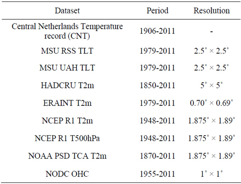
Table 1. Datasets used in this study, record length and horizontal resolution.
traction of both fits is similar (0.6 K in both cases), so by this means it is not possible to determine which fit is better. The uncertainty intervals of the regressions suggest that only the linear trend after 1980 is significant. However, according to the CPA analysis of the CNT temperature a change occurred in 1988 with a statistical significance of 100%, even when we increased the number of bootstraps to 5,000,000, which would make its significance > 99.9999%. Thus, according to the CPA the possibility of a shift around 1987-1988 is very real and cannot be excluded from a statistical point of view, with —according to the linear regressions—no statistically significant trends before and after 1987. Note that the CPA analysis did not detect any other change point in the CNT series with a significance level larger than 95%.
This result leads to several questions: did this shift occur in other European regions and if so, what was its spatial extent. And was this shift merely seen at the surface or also aloft?
To answer these questions, we applied the CPA to a range of temperature records representative for the location of the Netherlands obtained from gridded surface temperature reconstructions (HADCRU), to reanalysis data (ERA INTERIM, NCEP, NOAA) and satellite data (MSU from UAH and RSS. Figure 1(b) shows the time series of all datasets mentioned above for the grid box closest to the CNT location. The statistics of the CPA are summarized in Table 2. All datasets clearly identify a change in 1987 or 1988 at the CNT location with high confidence (significance levels vary between 99.1 and 100%), which is not surprising given the correspondence between the temperature anomalies during the period 1979-2010. We thus conclude that the possible 1987- 1988 European Climate Shift is a robust feature in the various datasets.
Before continuing with the analysis of spatial patterns of change points, a few remarks are in place with regard to the CPA methodology. First of all, confidence intervals to some extent depend on the length of the record. For example, the confidence level of the ECS is 100% for the full 1906-2011 CNT record. However, taking only the period 1979-2011, a shift is still detected in 1987 but with a confidence level of “only” 98.5%. The reduced confidence level is related to the fact that for the longer period the algorithm has a better estimate of what the undisturbed variability of the temperature record is. Furthermore, the confidence levels themselves are subject to some uncertainty. Taking a larger bootstrap sample of 10,000 rather than 1000 for the CNT series from 1979- 2011 leads to a confidence level of 98.3%, rather than the 98.5% for the 1000 bootstraps. These results indicate that some care has to be taken with the interpretation of significance levels.
4. Regional and Global Change Point Patterns
Given the presence of a change point in the various temperature records for the Netherlands, the next question is what the spatial extent of this change is. Figure 2 shows the locations around Europe where a change point was identified in various datasets for 1987 or 1988 and where confidence intervals are larger than 95%. There is a clear agreement among all datasets that the temperature change around 1987-1988 is not a localized but rather a
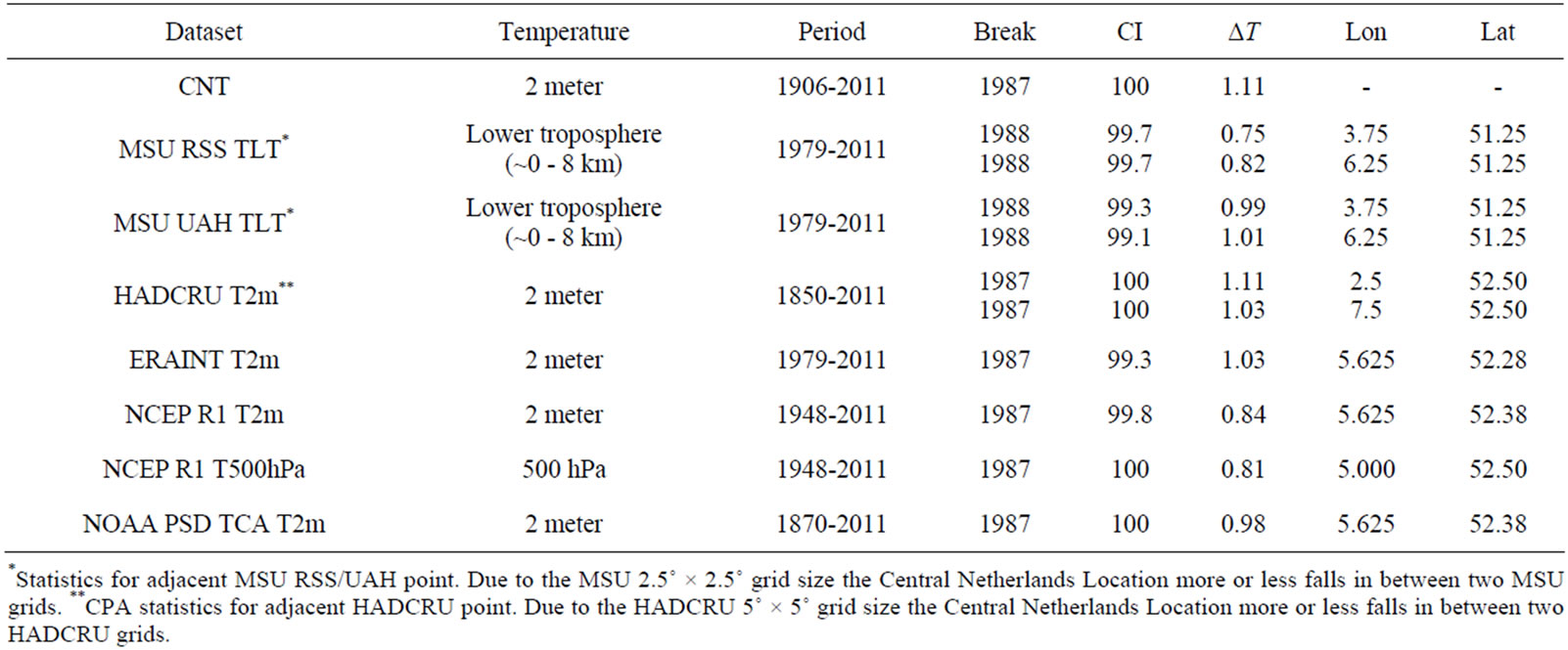
Table 2. Statistics of the 1987-1998 European Climate Shift as derived from the CUSUM algorithm. Indicated are the dataset, temperature altitude, record length, break year, confidence interval (CI) based on a 1000 member bootstrap (“without replacement”), temperature difference between the periods before and after the change (ΔT) and the geographical location of the dataset grid point closest to the Netherlands, in degrees East and North.
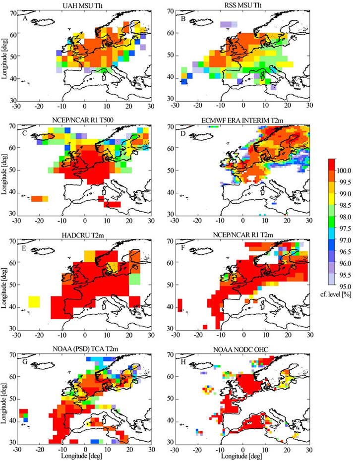
Figure 2. Spatial patterns of the statistical significance of the 1987-1988 ECS for the European domain. Only points with a significance larger than 95% are shown.
regional phenomenon, even visible in Ocean Heat Content data. The area of change stretches between the United Kingdom to central Europe and from the Alps and Pyrenees to southern Scandinavia, but depending on the dataset may include the Baltic area and northern Scandinavia, the northern Atlantic towards Iceland as well as the Iberian Peninsula and the western Mediterranean. Confidence levels are all highly significant, for most of the areas larger than 99%.
The presence of this robust and persistent area of change begs another question: are there other areas outside of Europe that also show a change point around 1987-1988. Figure 3 shows the global pattern of change points around 1987-1988 and with a confidence interval larger than 95%. Globally, we now see quite different spatial patterns among the various datasets. Both satellite
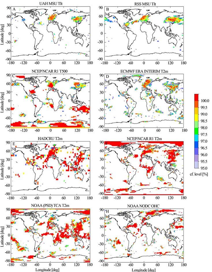
datasets (A,B) show only a few areas where a change is identified. Apart from Europe a change is identified over a large area in eastern Asia and western Pacific as well as some areas over the northern Atlantic Ocean around 30˚N. The latter is statistically less significant and the two satellite datasets are not in agreement on this. The other datasets agree on the European and East Asia change, but show much more scatter and some spatially coherent patterns not seen in the satellite data. The NCEP 500 hPa reanalysis data (C) shows changes in the subtropical Southern Hemisphere, in particular over Australia, and over Antarctica. The ECMWF ERA interim data (D) shows quite some additional “small scale scatter”. HADCRU (E) also shows quite some “scatter”. The NCEP reanalysis surface data (F) shows large scale changes in the Arctic as well as over equatorial Africa and over Antarctic. The NOAA TCA data (G) shows large signals in the Tropics and the Arctic, as well as smaller signals around the globe. The OHC (H), finally, also shows a strong Arctic signal and quite some scatter.
Given that the satellite data is—from a spatial point of view—the only record made with the same instrument, one interpretation of these findings is that all other records, either reconstructions or reanalysis data, suffer from inhomogeneities that contaminate long term records. On the other hand, all datasets agree on a Western Europe and an East Asia change, suggesting that both are real in a physical sense.
5. Discussion
The most important finding of our analysis is that a clear case can be made for a European Climate Shift around 1987-1988. All datasets analyzed here consistently show a change in mean temperature over Western Europe before and after 1987-1988, although the spatial extent of this shift varies among the various datasets. There also exists an apparent teleconnection with eastern Asia and the western Pacific, where also a shift is identified during this period.
An obvious legitimate question is what is causing the ECS and if there is a physical one at all. Variations in the NAO do not appear to have contributed much to recent warming in Europe [2] and the NAO is more important for high frequency (interannual) variability than for low frequency (decadal) variability [27].
Figure 4 shows the time series of three different NAO indices for the periods 1900-now and 1975-now. The one feature standing out is the high positive NAO indices in the late 1980’s and early 1990s, following a number of years in the mid 1980’s with of negative NAO values. It is well established that the winters of 1984/1985, 1985/ 1986 and 1986/1987 were cold in Western Europe which led to relatively low annual mean temperatures whereas the years after that (1988-1990) were all quite warm and that these temperature anomalies are related to variations in circulation patterns and thus the NAO [27]. On the other hand, the NAO index drops to more normal values during the 1990’s and thereafter, whereas the positive temperature anomaly remains. Furthermore, no changes in other modes of multidecadal internal climate variability like the Atlantic Multidecadal Oscillation (AMO), the Arctic Oscillation (AO), the Pacific Decadal Oscillation (PDO) and El Nino—Southern Oscillation (ENSO) have been reported around 1987-1988 [28,29]. Given that there has been a general upward trend in temperatures—possibly enhanced by strong reductions in aerosols over Europe, the so-called “brightening” [30]—it is likely that the accidental sequence of a few cold years followed by a few warm years under conditions of brightening results in a temperature sequence that in a statistical analysis is identified as a change point. This is consistent with the notion that NAO predominantly influences high frequency temperature variations, not long-term temperature variations [27]. Combined with the well established turnaround from “dimming” to “brightening” in the mid- 1980’s [27], we argue that the shift could actually be considered a fingerprint of European “brightening”. The detection of this climate shift should be viewed as a “spurious” result, i.e. not as a true physical shift in climate, despite its very high statistical significance (at least 5 sigma in our case). The occurrence of this spatial pattern thus could be a consequence of global anthropogenic greenhouse gas forcing, regional aerosol forcing and naturally occurring variations in atmospheric circulation patterns and is thereby fully consistent with the current understanding of the role of anthropogenic aerosols in explaining 20th century global warming [10].
One of the reasons that our statistical analysis results in such a high significance may be that autocorrelation properties of the time series is not preserved using the classical bootstrap method. A method to overcome this problem is to use a block bootstrap [31], in which blocks of data are resampled rather than individual measurement points. The use of blocks ensures that the autocorrelation properties of the data are preserved. The block length depends on the exact autocorrelation properties and can be estimated from the data, which in case of the CNT temperatures is six years. Testing for statistical significance using the block-bootstrap results in significance levels of approximately 97%, which is much smaller than the 5- sigma result from the traditional bootstrap. However, the block-bootstrap turns out to be unstable: the longer the block period, the smaller the statistical significance. Reason is that the CNT data contains one prominent change point, and selecting longer periods increases the possibility that the change point is resampled. This lack of stability indicates that for the time series at hand—non-stationary, autocorrelated and containing one change point— the block-bootstrap is not a suitable method for change point detection.
Further investigation of literature on the use of bootstrap methods suggests that in general no accepted bootstrap methods exist for non-stationary, autocorrelated time series containing change points [32]. On the other hand, Figure 1 shows that periods of three consecutive years with anomalously higher or lower temperatures do occur (for example 1907-1909; 1922-1924; 1940-1942; 1947-1949; 1959-1961 and 1974-1977). The frequent occurrence of such periods at least renders it possible or even plausible that such a sequence of events accidentally occurred around 1987-1988. Clearly more research is required from the perspective of statistics—in particular for auto correlated non-stationary time series containing change points.
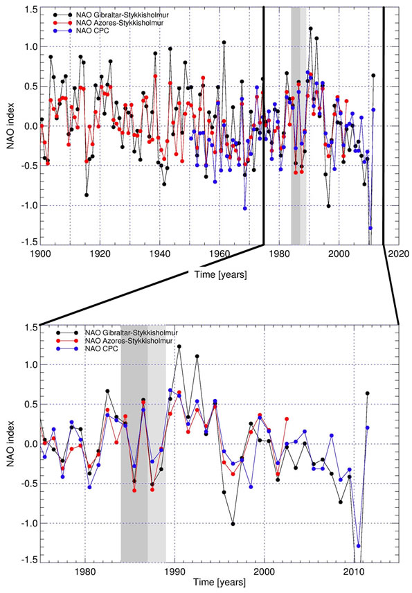
Figure 4. Time series of three North Atlantic Oscillation Indices [35,36]. The upper panel shows the period 1900-now, the lower panel a zoom-in for the period 1975-now. Indicates in grays are the years 1984-1987 (dark) and 1987-1988 (light).
Finally, the analysis of the spatial extent of the ECS also reveals reanalysis data, i.e. data based on many different measurement types and from different sources, suffering from discontinuities which seriously hamper the identification of change points in long records. This is not unexpected, as inhomogeneities in reconstructed data have been reported before [33,34]. However, from the perspective of sudden climate change and shifts in climate modes such contamination hampers the analysis of observational data.
REFERENCES
- G. J. van Oldenborgh, et al., “Western Europe Is Warming Much Faster than Expected,” Climate of the Past, Vol. 5, No. 1, 2009, pp. 1-12. doi:10.5194/cp-5-1-2009
- G. J. van Oldenborgh and A. P. van Ulden, “On the Relationship between Global Warming, Local Warming in the Netherlands and Changes in Circulation in the 20th Century,” International Journal of Climatology, Vol. 23, 2003, pp. 1711-1723. doi:10.1002/joc.966
- A. P. van Ulden and G. J. van Oldenborgh, “Large-Scale Atmospheric Circulation Biases and Changes in Global Climate Model Simulations and Their Importance for Climate Change in Central Europe,” Atmospheric Chemistry and Physics, Vol. 6, No. 4, 2006, pp. 863-881. doi:10.5194/acp-6-863-2006
- M. Reckermann, et al., “BALTEX—An Interdisciplinary Research Network for the Baltic Sea Region,” Envonmental Research Letters, Vol. 6, No. 4, 2011, Article ID: 045205.
- A. P. van Ulden, G. Lenderink, B. van den Hurk and E. van Meijgaard, “Circulation Statistics and Climate Change in Central Europe: Prudence Simulations and Observations,” Climatic Change, Vol. 81, No. S1, 2007, pp. 179-192. doi:10.1007/s10584-006-9212-5
- S. Keevallik, “Shifts in Meteorological Regime of the Late Winter and Early Spring in Estonia during Recent Decades,” Theoretical and Applied Climatology, Vol. 105, No. 1-2, 2011, pp. 209-215. doi:10.1007/s00704-010-0356-x
- S. Keevallik and T. Soomere, “Shifts in Early Spring Wind Regime in North-East Europe (1955-2007),” Climate of the Past, Vol. 4, No. 3, 2008, pp. 147-152. doi:10.5194/cp-4-147-2008
- A. Lehmann, K. Getzlaff and J. Harla, “Detailed Assessment of Climate Variability in the Baltic Sea Area for the Period 1958-2009,” Climatic Research, Vol. 46, 2011, pp. 285-196. doi:10.3354/cr00876
- G. van der Schrier, A. van Ulden and G. J. van Oldenborgh, “The Construction of a Central Netherlands Temperature,” Climate of the Past, Vol. 7, No. 2, 2011, pp. 527-542. doi:10.5194/cp-7-527-2011
- IPCC, “Summary for Policymakers,” In: Field, et al., Eds., Special Report on Managing the Risks of Extreme Events and Disasters to Advance Climate Change Adaptation, Cambridge University Press, Cambridge and New York, 2011. http://ipcc-wg2.gov/SREX/
- A. N. Pettitt, “A Simple Cumulative Sum Type Statistic for the Change-Point Problem with Zero-One Observations,” Biometrika, Vo. 67, No. 1, 1980, pp. 79-84. doi:10.1093/biomet/67.1.79
- W. A. Taylor, “Change-Point Analysis: A Powerful New Tool for Detecting Changes,” 2000. http://www.variation.com/cpa/tech/changepoint.html
- B. Efron and R. J. Tibshirani, “An Introduction to the Bootstrap,” Chapman and Hall, New York, 1993.
- J. Reeves, J. Chen, X. L. Wang, R. Lund and Q. Q. Lu, “A Review and Comparison of Change Point Detection Techniques for Climate Data,” Journal of Applied Meteorology and Climatology, Vol. 46, 2007, pp. 900-915. doi:10.1175/JAM2493.1
- J. R. Christy, W. B. Norris, R. W. Spencer and J. J. Hnilo, “Tropospheric Temperature Change Since 1979 from Tropical Radiosonde and Satellite Measurements,” Journal of Geophysical Research—Atmospheres, Vol. 112, No. 6, 2007, Article ID: D06102. doi:10.1029/2005JD006881
- C. A. Mears and F. J. Wentz, “Construction of the RSS V3.2 Lower-Tropospheric Temperature Dataset from the MSU and AMSU Microwave Sounders,” Journal of Atmospheric Oceanic Technology, Vol. 26, No. 8, 2009, pp. 1493-1509. doi:10.1175/2009JTECHA1237.1
- E. Kalnay, et al., “The NCEP/NCAR 40-Year Reanalysis Project,” Bulletin of the American Meteorological Society, Vol. 77, No. 3, 1996, pp. 437-470. doi:10.1175/1520-0477(1996)077%3C0437:TNYRP%3E2.0.CO;2
- D. P. Dee, et al., “The ERA-Interim Reanalysis: Configuration and Performance of the Data Assimilation System,” Quarterly Journal of the Royal Meteorological Society, Vol. 137, No. 656, 2011, pp. 553-597. doi:10.1002/qj.828
- P. D. Jones, M. New, D. E. Parker, S. Martin and I. G. Rigor, “Surface Air Temperature and Its Variations over the Last 150 Years,” Reviews in Geophysics, Vol. 37, No. 2, 1999, pp. 173-199. doi:10.1029/1999RG900002
- N. A. Rayner, et al., “Globally Complete Analyses of Sea Surface Temperature, Sea Ice and Night Marine Air Temperature, 1871-2000,” Journal of Geophysical Research— Atmospheres, Vol. 108, No. D14, 2003, Article ID: 4407. doi:10.1029/2002JD002670
- N. A. Rayner, et al., “Improved Analyses of Changes and Uncertainties in Marine Temperature Measured in Situ Since the Mid-Nineteenth Century: The HadSST2 Dataset,” Journal of Climate, Vol. 19, 2006, pp. 446-469. doi:10.1175/JCLI3637.1
- P. Brohan, J. J. Kennedy, I. Harris, S. F. B. Tett and P. D. Jones, “Uncertainty Estimates in Regional and Global Observed Temperature Changes: A New Dataset from 1850,” Journal of Geophysical Research—Atmospheres, Vol. 111, 2006, Article ID: D12106. doi:10.1029/2005JD006548
- J. S. Whitaker, G. P. Compo, X. Wei and T. M. Hamill, “Reanalysis without Radiosondes Using Ensemble Data Assimilation,” Monthly Weather Review, Vol. 132, No. 5, 2004, pp. 1190-1200. doi:10.1175/1520-0493(2004)132%3C1190:RWRUED%3E2.0.CO;2
- G. P. Compo, J. S. Whitaker and P. D. Sardeshmukh, “Feasibility of a 100-Year Reanalysis Using Only Surface Pressure Data,” Bulletin of the American Meteorological Society, Vol. 87, No. 2, 2006, pp. 175-190. doi:10.1002/qj.776
- G. P. Compo, et al., “The Twentieth Century Reanalysis Project,” Quarterly Journal of the Royal Meteorological Society, Vol. 137, No. 654, 2009, pp. 1-28. doi:10.1002/qj.776
- S. Levitus, S. I. Antonov, J. L. Antonov, T. P. Boyer, R. A. Locamini and H. E. Garcia, “Global Ocean Heat Content 1955-2008 in Light of Recently Revealed Instrumentation Problems,” Geophysical Research Letters, Vol. 36, No. 7, 2009, Article ID: L07608. doi:10.1029/2008GL037155
- M. Chiacchio and M. Wild, “Influence of NAO and Clouds on Long-Term Seasonal Variations of Surface Solar Radiation in Europe,” Journal of Geophysical Research—Atmospheres, Vol. 115, No. D4, 2010, Article ID: D00D22. doi:10.1029/2009JD012182
- G. Foster and S. Rahmstorf, “Global Temperature Evolution 1979-2010,” Environmental Research Letters, Vol. 6, 2011, Article ID: 044022. doi:10.1088/1748-9326/6/4/044022
- T. DelSole, M. K. Tippett and J. Shukla, “A Significant Component of Unforced Multidecadal Variability in the Recent Acceleration of Global Warming,” Journal of Climate, Vol. 24, No. 3, 2010, pp. 909-926.
- M. Wild, “Global Dimming and Brightening: A Review,” Journal of Geophysical Research—Atmospheres, Vol. 114, No. D10, 2009, Article ID: D00D16. doi:10.1029/2008JD011470
- M. Mudelsee, “Climate Time Series Analysis, Classical Statistical and Bootstrap methods,” Atmospheric and Oceanographic Sciences Library, Springer, New York, 2010.
- S. Smeekes, “Bootstrapping Nonstationary Time Series,” Ph.D. Thesis, Maastricht Research School of Economics of Technology and Organizations, Maastricht University, The Netherlands, 2009.
- A. Sterl, “On the (In) Homogeneity of Reanalysis Products,” Journal of Climate, Vol. 17, No. 19, 2004, pp. 3866-3873. doi:10.1175/1520-0442(2004)017%3C3866:OTIORP%3E2.0.CO;2
- J. A. Screen and I. Simmonds, “Erroneous Arctic Temperature Trends in the ERA-40 Reanalysis: A Closer Look,” Journal of Climate, Vol. 24, No. 10, 2011, pp. 2620-2627. doi:10.1175/2010JCLI4054.1
- P. D. Jones, et al., “Extension to the North Atlantic Oscillation Using Early Instrumental Pressure Observations from Gibraltar and South-West Iceland,” International Journal of Climatology, Vol. 17, 1997, pp. 1433-1450.
- A. G. Barnston and R. E. Livezey, “Classification, Seasonality and Persistence of Low-Frequency Atmospheric Circulation Patterns,” Monthly Weather Review, Vol. 115, 1987, pp. 1083-1126.
NOTES
*Corresponding author.