Atmospheric and Climate Sciences
Vol. 2 No. 3 (2012) , Article ID: 21395 , 9 pages DOI:10.4236/acs.2012.23027
Prospects for Improving the Operational Seasonal Prediction of Tropical Cyclone Activity in the Southern Hemisphere
1National Climate Centre, Australian Bureau of Meteorology, Melbourne, Australia
2School of Mathematical and Geospatial Sciences, Royal Melbourne Institute of Technology (RMIT) University, Melbourne, Australia
3Centre for Australian Weather and Climate Research, Australian Bureau of Meteorology, Melbourne, Australia
Email: Y.Kuleshov@bom.gov.au
Received March 7, 2012; revised April 20, 2012; accepted May 12, 2012
Keywords: Tropical Cyclones; Seasonal Prediction; Australian Region
ABSTRACT
Tropical cyclones (TCs) are the most destructive weather phenomena to impact on tropical regions, and reliable prediction of TC seasonal activity is important for preparedness of coastal communities in the tropics. In investigating prospects for improving the skill of TC seasonal prediction in the South Indian and South Pacific Oceans, including the Australian Region, we used linear regression to model the relationship between the annual number of cyclones and three indices (SOI, NIÑO3.4 and 5VAR) describing the strength of the El Niño-Southern Oscillation (ENSO). The correlation between the number of Australian Region (90˚E - 160˚E) TCs and the indices was strong (3-month 5VAR −0.65, NIÑO3.4 −0.62 and SOI +0.64), and a cross-validation assessment demonstrated that the models which used July-August-September indices and the temporal trend as the predictors performed well. The predicted number of TCs in the Australian Region for 2010/2011 and 2011/2012 seasons was 14 (11 recorded) and 12, respectively. We also found that the correlation between the numbers of TCs in the western South Indian region (30˚E to 90˚E) and the eastern South Pacific region (east of 170˚E) and the indices was weak, and it is therefore not sensible to build linear regression forecast models for these regions. We conclude that for the Australian Region, the new statistical model provides prospects for improvement in forecasting skill compared to the statistical model currently employed at the National Climate Centre, Australian Bureau of Meteorology. The next step towards improving the skill of TC seasonal prediction in the various regions of the Southern Hemisphere will be undertaken through analysis of outputs from the dynamical climate model POAMA (Predictive Ocean-Atmosphere Model for Australia).
1. Introduction
Tropical cyclones (TCs) are the most destructive weather phenomena to impact on tropical regions. Reliable prediction of seasonal TC activity is important for preparedness of coastal communities of Australia and island nations in the Pacific and Indian Oceans ahead of the coming cyclone season. Over recent decades, statistical model-based methods for prediction of TC activity in the coming season have been developed for a number of regions in various ocean basins, starting with the pioneering work of Gray [1]. Statistical models explore relationships between large-scale environmental drivers which modulate TC activity, for example the El Niño-Southern Oscillation (ENSO) phenomenon, and observed numbers of TCs to derive linear regression equations which can be used for prediction of future cyclone activity. Indices such as the Southern Oscillation Index (SOI) and sea surface temperatures (SSTs) in some oceanic areas are commonly used to build such statistical models. However, there are two major constraints associated with the statistical model-based approach. Firstly, accurate historical cyclone records (ideally records covering a reasonably long period of time) are required. Secondly, in a globally warming environment, statistical relationships based on historical data may not produce reliable results when values of the environmental indices are outside of the range of historical records.
The availability of satellite imagery has significantly improved our knowledge of TCs, with satellite remote sensing being vital for accurate estimates of parameters such as TC position (e.g., the location of minimum atmospheric pressure) and TC intensity, however with the latter to a lesser degree of confidence compared to estimating TC position [2]. Satellite images are used by forecasters for preparing operational (real-time) and besttrack data, and a complete digital Geostationary Meteorological Satellite (GMS) archive for the Southern Hemisphere has been prepared at the Australian Bureau of Meteorology for use in TC reanalysis [3]. Thus, TC historical records for the Southern Hemisphere, at least in terms of the annual number of cyclone occurrences, are of high quality for the “satellite era”—that is from early 1970s [2,4,5].
Utilising historical data for the Australian region, Nicholls [6] examined interannual variability in TC activity, and demonstrated a link between ENSO and inter-seasonal variations in TC numbers. The TC-ENSO relationship was used in developing statistical methodology for forecasting seasonal TC activity in the Australian and some other regions in subsequent studies (e.g., [7-9]). In general, such a methodology of statistical seasonal forecasting of seasonal cyclone numbers ahead of the season (November to April in the Southern Hemisphere) employs ENSO indices (e.g., the SOI which describes the state of the atmospheric circulations, or the NIÑO4 and NIÑO3.4 SST anomaly indices) for months which precede the TC season (e.g., a three-month average for August, September and October). These models performed reasonably well over past years; however, during the 2010-2011 TC season, which corresponded to a very strong La Niña event, the statistical models signifycantly over-predicted the number of TCs in the Australian region.
The 2010-2011 Australian region cyclone season was actually a near-average tropical cyclone season, with eleven tropical cyclones forming compared to an average of 12. However, the seasonal forecast issued by the Bureau of Meteorology’s National Climate Centre (NCC) ahead of the season for the Australian region (the area south of the equator, 90˚E to 160˚E) predicted on the basis of strong La Niña conditions that the basin could turn into the most active season since 1983/1984, with 20 - 22 tropical cyclones developing in or moving into the region [10]. Similarly, the Guy Carpenter Asia-Pacific Climate Impact Centre (GCACIC) at the City University of Hong Kong has issued a forecast that predicted that 19 TCs would either develop within or move into the basin [11].
Thus, a motivation for this study was to investigate prospects for improving the skill of operational seasonal prediction of TC activity in the regions of the Southern Hemisphere using statistical model-based approaches. In respect of this, the new best track TC database for the Southern Hemisphere described in the next section of this paper is used for the analysis of historical TC data. The statistical prediction models developed are presented in Section 3. This is followed by a discussion and conclusions in the final section.
2. Data and Methodology
A TC archive for the Southern Hemisphere has been prepared at the NCC in the Australian Bureau of Meteorology in close collaboration with international partners [2]. The archive is a result of multinational efforts of the National Meteorological and Hydrological Services from the Southern Hemisphere nations and has been derived from several data sources. The data for the western South Indian Ocean (30˚E to 90˚E) have been provided by Météo-France (La Réunion), for the Australian region (90˚E to 160˚E) by the Australian Tropical Cyclone Warning Centres (Brisbane, Darwin and Perth), and for the eastern South Pacific Ocean (east of 160˚E) by the Meteorological Services of Fiji and New Zealand. TC tracks from these archives were merged into one archive, ensuring consistency of track data when TCs cross regional borders. The data from the Southern Hemisphere TC archive are available from the Pacific Tropical Cyclone Data Portal (http://www.bom.gov.au/cyclone/history/tracks).
The time series of TC annual occurrences in the Australian region is presented in Figure 1. To keep consistency with results of our previous studies, the genesis of a TC is defined when a cyclonic system first attains a central pressure equal to or less than 995 hPa. Primary focus of the study is the Australian region, however, prospects to develop skillful statistical models for TC seasonal forecasting in the eastern South Pacific Ocean and the western South Indian Ocean were also investigated.
A linear regression model technique was used to model the relationship between the number of cyclones in three regions of the Southern Hemisphere. Studies by Ramsay et al. [12] and Kuleshov et al. [8] demonstrated a strong correlation (about −0.7) between the annual number of TCs in the Australian region and the August-September-October-averaged NIÑO4 and NIÑO3.4 indices, with some other ENSO indices also showing high correlation. For the eastern South Pacific Ocean, the NIÑO3.4, SOI and 5VAR indices correlated with the TC number better than other ENSO indices [8].
The NIÑO3.4 and the SOI are the two most commonly used indices in defining ENSO phases. The SOI data used in this study were obtained from the Australian Bureau of Meteorology and are available on its website at www.bom.gov.au/climate/current/soihtm1.shtml. Values for the NIÑO3.4 (SST anomalies in Niño3.4 region, 3-month running mean) were obtained from the Climate Prediction Center, NOAA (ftp.cpc.ncep.noaa.gov/wd52dg/ data/indices/sstoi.indices). A multivariate ENSO index, based on the first principal component of monthly Darwin
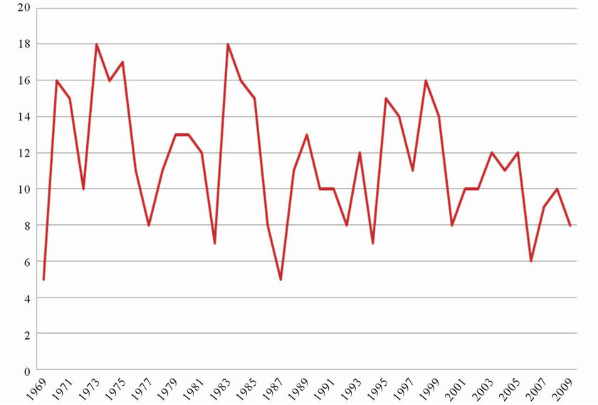
Figure 1. Time series of TC annual occurrences in the Australian region for the 1969/1970 to 2009/2010 seasons.
mean sea level pressure (MSLP), Tahiti MSLP, and the NIÑO3, NIÑO3.4 and NIÑO4 SST indices, has been developed at the NCC (see also [5,8]). Its base period is 1950-1999. Strength of a multivariate index is in integrating both atmospheric and oceanic responses to changes in the ENSO phases in one index. We denote this standardised monthly anomaly index as the 5VAR index. In this study, the NIÑO3.4, the SOI and the 5VAR indices were used for further investigation of the TC-ENSO relationship.
3. Results
3.1. Correlation between the Annual Number of TCs and the ENSO Indices
The correlation coefficient was calculated between the annual number of TCs and the three selected indices for each month of two consecutive years in which the TC season is included. Thus, we measure a degree of correlation between the number of cyclones in the TC season with the indices before, during and after the TC season. For each index, there would be twenty-four correlation coefficients for individual months denoted as January (t), February (t),  , December (t), January (t + 1),
  and December (t + 1), where t is the year in which the cyclone season starts. We also investigated the correlation by averaging values of the ENSO indices for m neighbouring months, where m takes values 2 and 3. The higher the values of m, the less importance is given to individual monthly values of the index as equal weights are given to each of the m months. The correlation between annual number of TCs in the Australian region and the monthly 5VAR, NIÑO3.4 and SOI indices is presented in Figure 2 (for the SOI, correlations with –SOI are plotted for consistency of sign with the other indices).
In agreement with earlier studies, the best correlation is found for the months from August, A (t), to January of the next year, J (t + 1). While the 5VAR and NIÑO3.4 indices demonstrate high correlation in a range from −0.6 to −0.7 for six months from A (t) to J (t + 1), the SOI has the strongest correlation in A (t) (−0.62) which then decreases to less than −0.5 from October, O (t), onwards. It appears that the state of the atmosphere alone (as described by the SOI) is an important contributor to the environment in which TCs form early in the season, but not as important as ocean (or combined contribution of ocean and the atmosphere as described for example by 5VAR) during the TC season.
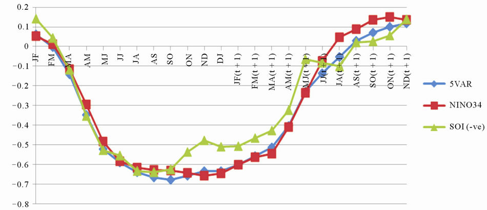
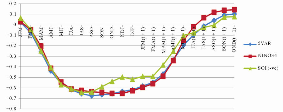
The correlation coefficients were also computed for two-month and three-month averages (Figures 3 and 4, respectively). Similar conclusions can be drawn from the analysis of the correlation of the TC number with biand tri-monthly averaged ENSO indices. The highest correlation was found for the averages that include A (t) up to those that include J (t + 1) (although still with the exception of the SOI).
A TC seasonal forecast for the regions of the Southern Hemisphere is typically issued in October, prior to the
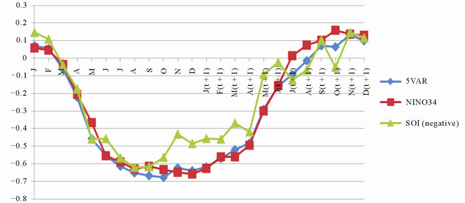
Figure 2. The correlation between annual number of TCs in the Australian region and the monthly 5VAR, NIÑO3.4 and SOI indices.
beginning of the TC season. As monthly-averaged values of the ENSO indices are usually available in the second week of the following month, for the prediction model to be implemented operationally the values for the months beyond September cannot be used. Consequently, in Table 1 we present the highest correlation coefficient of the total annual number of TCs in the Australian region with the three ENSO indices examined and the corresponding months that have been averaged only for months prior to October. Note that the highest correlations for the entire 24-month period examined are only marginally higher for the months beyond September. For example, in the case of the 2-month average for the 5VAR index, the strongest correlation of −0.678 arises from the average of the September and October values, while the correlation arising from the average of August and September values (presented in the table) is −0.665.
As can be seen from the table, the 5VAR performs better than other two indices examined demonstrating the strongest monthly, bi-monthly and tri-monthly correlation. Inspecting the correlations of each index, we found that the strongest correlation for the 5VAR is one month pre-season September, while it is the two-month average of August and September for NIÑO3.4 and the threemonth average of July, August and September for the SOI (shown in bold font in Table 1). Based on these finding, models were built for each of the indices using the appropriate m-month averages of the data.
3.2. Multiple Regression Models
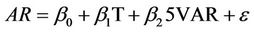
We modified the simple linear regression model developed earlier in [8] by adding a temporal trend variable (T) as one of the predictors. The candidate models are Model 1
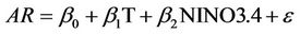
Model 2
Model 3
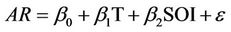
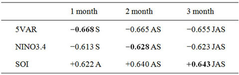
Table 1. The highest correlation coefficients between the annual number of TCs in the Australian region and the monthly, bi-monthly and tri-monthly 5VAR, NIÑO3.4 and SOI indices. Letters following the numerical values denote which months or combinations of months are used.
where e denotes the noise variable, assumed to be normally distributed with mean 0 and variance s2, i.e., e~N (0,σ2).
It was found that all three models have significant coefficients for the three indicial predictors. The assumptions of randomly and normally distributed residuals are also satisfied. Although the temporal predictor is not statically significant for the first two models (although not far from being statistically significant), the adjusted values R2 for all three models have increased by comparing with our earlier model without the temporal trend. The adjusted values R2 for the model with the 5VAR as a predictor has increased from 0.432 to 0.452, while R2 increased from 0.3791 to 0.4005 for the NIÑO3.4 models. As for the model with SOI as a predictor, the temporal predictor is marginally significant at the 10% significance level, the percentage of explained variation has increased from 0.4063 to 0.4462. As in our earlier study, the regression model with 5VAR as the predictor surpasses the other two models with SOI or NIÑO3.4 as the predictors.
In our analyses, we also take into account an influential point, which is an observation that greatly affects the slope of the regression line. Observations can be flagged as potential influential points by means of leverage points, DFFITS and Cook’s distance. The cut off point for leverage in the above three models is 0.0487, but note that a leverage point is not always an influential point. DFFITS is a diagnostic meant to show how influential a point is in a statistical regression [13]. It is defined as the change (“DFFIT”), in the predicted value for a point, obtained when that point is left out of the regression, “Studentized” by dividing by the estimated standard deviation of the fit at that point:
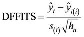
where  and
and  are the prediction for point i with and without point i included in the regression, s(i) is the standard error estimated without the point in question, and hii is the leverage for the point. Large values of DFFITS indicate influential observations. An observation with DFFITS value greater than 0.453 is flagged for scrutiny. As for Cook’s distance, an observation is also flagged if the value is greater than 1.
In our analyses, the following observations were flagged as potential influential points:
Model 1: Observations 1, 20 and 29Model 2: Observations 1 and 29, and Model 3: Observations 1 and 20.
Model 1 was then adjusted and fitted three times, each time omitting one flagged observation and the same was done with Models 2 and 3 by excluding observations 20 and 29 alternatively. The models with the highest adjusted R2 values were kept separately from Models 1, 2 and 3. In order to detect if any multi-collinearity problems are present in the above models, VIF (Variance inflation factor) was also calculated. The results (not shown) demonstrated that there were no multi-collinearity problems in the proposed multiple regression models.
The first observation, five TCs in the 1969/1970 season, was found to be the most influential point for all three models. All three indices along with the temporal trend explained 44% to 50% of the total variation in the annual number of TCs in the Australian region. After removing the influential point, one can see that all three modified regression models perform better in terms of improved adjusted R2 values. The temporal trend effect also became significant (P-values < 0.05) after removing the first observation, making the temporal trend an essential predictor for the annual number of TCs in Australian region.
One of the possible reasons for TC donward trend in the Australian region could be due to ENSO impact on TC geographical distribution. In the Australian region, a reduction in TC activity is usually observed in El Niño years, while in La Niña years TC activity is typically higher compared to El Niño years [5,14]. In 1970s, four La Niña events and four El Niño events were identified, while during the next three decades only five La Niña events were observed, with 12 El Niño events recorded [8]. Such distribution in frequency of the ENSO cold and warm phases is one of the plausible reasons for the observed downward trend in TCs in the Australia regions. This trend could also reflect a slow periodicity in TC variability due to variation in major climatic drivers with a period rather longer than the study period (see, for example, impact of the Pacific Decadal Oscillation on TC variability over the western North Pacific described in [15]). Thus, incorporation of a temporal trend in the statistical model requires its regular revision, perhaps annually, accounting for TC activity in the last season and adjusting the model accordingly.
By comparing with the simple linear regression counterparts in [8], all the developed models have improved performance. For example, the model using SOI as a predictor was not the best model in our earlier study with the adjusted R2 of about 40%, while in the current analyses the model demonstrates an improvement in modelling the annual number of TCs with the R2 reaching 50%.
Cross-validation was employed to assess the models’ performance, each time leaving one observation out and validating the analysis on that single observation. The RMSE (root mean squared error) was calculated as the measurement of fit. RMSEs were 2.72, 2.86 and 2.70 for the Models 1.1 (5VAR), 2.1 (NIÑO3.4) and 3.1 (SOI), respectively. The cross-validation results are in agreement with those using adjusted R2 as the model assessment criteria, that is, the models which used the preseason July-August-September SOI and September 5VAR indices and the time trend as the predictors demonstrated the best performance.
Using the developed models, the modelled annual number of TCs in the Australian region was compared with the observed (Figure 5).
Using the developed models, forecast of a number of TCs in the Australian region in 2010/11 was prepared
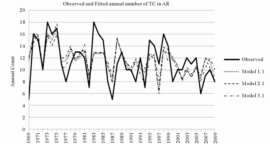
Figure 5. Time series of the total annual number of TCs in the Australian region as observed (solid line) and predicted using the 5VAR index + Time (Model 1.1), NIÑO3.4 index + Time (Model 2.1) and the SOI index + Time (Model 3.1).
(Table 2), with the standard error (SE) of the forecast given in brackets. The predicted number averaged over the three models is 14, which is higher than the observed number of 11 cyclones; however the models demonstrate improvement in prediction skill compared to the statisticcal models currently used by the NCC which predicted 20 to 22 cyclones.
The forecast for the number of TCs in 2011/2012 was also prepared using the three models. The numbers are similar for all three models and they indicate that the predicted TC activity in the Australian region for 2011/2012 cyclone season, 12 cyclones averaged over the three models, is expected to be similar to the longterm average of 12 cyclones.
Regression analysis for the eastern South Pacific Ocean and the western South Indian Ocean was also performed. Correlation between a number of TCs in the regions and the ENSO indices was calculated for the 1-, 2- and 3-month average. For each index, the month (months) with the highest correlation with the number of TCs in the region were selected. It was found that the correlations were not as strong as in the Australian region. For example, in the eastern South Pacific Ocean the strongest relationship with the number of TCs was found for September indices, although the association was weak (0.297 for the 5VAR, 0.318 for the NIÑO3.4 and 0.273 for the SOI). With these weak correlations, we conclude that it is not sensible to further build linear regression models.
3.3. Statistical-Dynamical Model-Based Approach for TC Seasonal Prediction
The Australian Bureau of Meteorology has developed a dynamical climate prediction model POAMA (Predictive Ocean-Atmosphere Model for Australia) [16]. It has been demonstrated that POAMA has substantial skill in predicting SSTs and rainfall across the Asia-Pacific region [17]. The skill results indicate the potential for developing TC seasonal prediction using statistical-dynamical model-based approach. Developing the improved statistical regression models, we found that the 5VAR index demonstrated the best correlation with the TC number and the correlation was constantly high (close to 0.7 in the Australia region) for six months from August, A (t), to
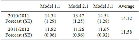
Table 2. Forecasts of the number of TCs occurring in the Australian region in 2010/11 and 2011/12 prepared using the developed models.
January of the next year, J (t + 1) (Section 3.1). It leads us to a proposition that using outputs from the dynamical model POAMA obtained prior to the TC season, it is possible to compute predicted values for the ENSO indices in advance (e.g. POAMA outputs generated in August and September can be used to compute October-November-December 5VAR values) and then use a statistical model to predict TC number. This approach may be particularly beneficial for early warning of expected active TC season (issued 1 - 2 months ahead of the statistical model-based forecast). In this study, we simulated such approach by the development of a regression model using October-November-December values of the 5VAR index as a predictor. Similar to the results in Section 3.2, the model with additional time trend has better performance than having 5VAR index only as the single explanatory variable.
There were four observations flagged as potential influential points in our proposed model, and they were observations 1, 20, 29 and 39. The models were re-built iteratively each time by omitting one flagged observation, and the model that excludes the first observation (1969/1970 season) was retained due to its highest adjusted R2 value (0.4932). The results are given in Table 3. One can see that both the 5VAR index and time trend are significant at 5% level of significance in the model.
The forecast of the number of TCs was also derived based on the developed model with the values of October-November-December 5VAR index in 2010. The resulting predicted number of TCs in the Australian region in 2010/2011 is 13.45, with the standard error 1.11. The obtained results of our pilot study for possible application of statistical-dynamical model-based approach encourage us to continue this investigation using POAMA outputs which we aim to conduct in our subsequent study.
4. Discussion and Conclusions
Interannual variability in the intensity and distribution of TCs is large, and presently greater than any trends that are ascribable to climate change. Historically TCs have had major impacts on agriculture, water supplies, safety and economic wellbeing of Australia and island countries of the South Pacific and South Indian Oceans. Better managing the year to year variability in cyclones is a practical means for decreasing current and future
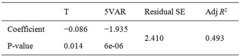
Table 3. Multiple linear regression with both time trend and the October-November-December 5VAR.
vulnerability to TCs. In addition, understanding the drivers of variability provides greater confidence in future predictions and projections. This is particularly important as the current understanding of TCs and seasonal conditions is mainly drawn from historical data and past covariability with drivers such as the ENSO, which are less valid in a changing climate. One issue that has emerged is a problem in predicting TC occurrence based on historical relationships, with predictors such as the SOI and SSTs now frequently lying outside of the range of past variability which was demonstrated by over-predicting TC activity in the Australian region for 2010/2011 TC season.
Currently, a statistical model-based prediction of TC activity in the coming season is used by the NCC for operational seasonal forecasting in the Australian region and the Pacific. Statistical models are also used by other agencies, for example the National Institute for Water and Atmospheric Research (NIWA) in New Zealand and the GCACIC, Hong Kong. In this study, we demonstrated a possibility of improving the accuracy of seasonal forecasts in the Australian region using statistical model-based approach. However, we also found that statistical models cannot produce skilful forecast of TC activity for other regions of the Southern Hemisphere.
We also made a first step towards investigating a possibility to apply statistical-dynamical model-based approach for TC seasonal prediction. The statistical models are based on historical climate data. Consequently, it leads to shortcomings because the statistical models cannot account for aspects of climate variability and change that are not represented in the historical record. This is an increasing problem as climate change brings new and unforeseen climate conditions. Dynamical (physics-based) climate models do not have this short-coming and are consequently better at incorporating the effects of a changing climate, whatever its character or cause. Therefore, the transition from a statistical to a dynamical prediction system will ultimately provide more valuable and applicable climate information about tropical cyclone seasonal variability, which can inform decision making, responses and adaptation in Australia and Pacific and Indian Ocean island countries. High-quality TC seasonal prediction also enables to move to a lesser reliance on historical climatologies which can give misleading information about the to-be-expected climate conditions and the likelihood of extreme events.
We conclude that for the Australian region the developed statistical models demonstrate improvement in forecasting skill compared to the currently employed NCC model. The next step towards improving skill of TC seasonal prediction in the regions of the Southern Hemisphere will be undertaken through the direct analysis of outputs from the dynamical climate models such as POAMA.
5. Acknowledgements
The research discussed in this paper was conducted with the partial support of the Pacific-Australia Climate Change Science and Adaptation Planning program (PACCSAP), which is supported by the Australia Agency for International Development, in collaboration with the Department of Climate Change and Energy Efficiency, and delivered by the Bureau of Meteorology and the RMIT University.
REFERENCES
- W. M. Gray, “Hurricanes: Their Formation, Structure and likely Role in the Tropical Circulation,” In: D. B. Shaw, Ed., Supplement to Meteorology over the Tropical Oceans, James Glaisher House, Bracknell, 1979, pp. 155-218.
- Y. Kuleshov, R. Fawcett, L. Qi, B. Trewin, D. Jones, J. McBride and H. Ramsay, “Trends in Tropical Cyclones in the South Indian Ocean and the South Pacific Ocean,” Journal of Geophysical Research, Vol. 115, 2010, 9 pages. doi:10.1029/2009JD012372
- M. Broomhall, I. Grant, L. Majewski, M. Willmott, D. Jones and Y. Kuleshov, “Improving the Australian Tropical Cyclone Database: Extension of GMS Satellite Image Archive,” In: Y. Charabi, Ed., Indian Ocean Tropical Cyclones and Climate Change, Springer, New York, 2010, pp. 199-206. doi:10.1007/978-90-481-3109-9_24
- G. J. Holland, “On the Climatology and Structure of Tropical Cyclones in the Australian/Southwest Pacific Region: I. Data and T. Storms,” Australian Meteorological Magazine, Vol. 32, No. 1, 1984, pp. 1-15.
- Y. Kuleshov, L. Qi, R. Fawcett and D. Jones, “On Tropical Cyclone Activity in the Southern Hemisphere: Trends and the ENSO Connection,” Geophysical Research Letters, Vol. 35, 2008, 5 pages. doi:10.1029/2007GL032983
- N. Nicholls, “A Possible Method for Predicting Seasonal Tropical Cyclone Activity in the Australian Region,” Monthly Weather Review, Vol. 107, No. 9, 1979, pp. 1221- 1224. doi:10.1175/1520-0493(1979)107<1221:APMFPS>2.0.CO;2
- N. Nicholls, “Recent Performance of a Method for Forecasting Australian Seasonal Tropical Cyclone Activity,” Australian Meteorological Magazine, Vol. 40, No. 2, 1992, pp. 105-110.
- Y. Kuleshov, L. Qi, R. Fawcett and D. Jones, “Improving Preparedness to Natural Hazards: Tropical Cyclone Prediction for the Southern Hemisphere,” In: J. Gan, Ed., Advances in Geosciences, World Scientific Publishing, Singapore City, 2009, pp. 127-143.
- K. S. Liu and J. C. L. Chan, “Interannual Variation of Southern Hemisphere Tropical Cyclone Activity and Seasonal Forecast of Tropical Cyclone Number in the Australian Region,” International Journal of Climatology, Vol. 32, No. 2, 2010, pp. 190-202. doi:10.1002/joc.2259
- NCC, “2010/11 Australian Tropical Cyclone Seasonal Outlook,” 2010. http://www.webcitation.org/5tYr6op9uRetrieved2011-11-11
- GCACIC, 2010. http://weather.cityu.edu.hk/tc_forecast/2010_forecast_NOV.pdf Retrieved 2011-11-11
- H. A. Ramsay, L. M. Leslie, P. J. Lamb, M. B. Rickman and M. Leplastrier, “Interannual Variability of Tropical Cyclones in the Australian Region: Role of Large-Scale Environment,” Journal of Climate, Vol. 21, No. 5, 2008, pp. 1083-1103. doi:10.1175/2007JCLI1970.1
- D. A. Belsley, K. Edwin and E. W. Roy, “Regression Diagnostics: Identifying Influential Data and Sources of Collinearity,” Wiley Series in Probability and Mathematical Statistics, John Wiley & Sons Ltd., New York, 1980.
- N. Nicholls, C. W. Landsea and J. Gill, “Recent Trends in Australian Region Tropical Cyclone Activity,” Meteorology and Atmospheric Physics, Vol. 65, No. 3-4, 1998, pp. 197-205. doi:10.1007/BF01030788
- K. S. Liu and J. C. L. Chan, “Interdecadal Variability of Western North Pacific Tropical Cyclone Tracks,” Journal of Climate, Vol. 21, No. 17, 2008, pp. 4464-4476. doi:10.1175/2008JCLI2207.1
- G. Wang, O. Alves, D. Hudson, H. Hendon, G. Liu and F. Tseitkin, “SST Skill Assessment from the New POAMA- 1.5 System,” BMRC Research Letter, No. 8, 2008.
- H. H. Hendon, E. Lim, G. Wang, O. Alves and D. Hudson, “Prospects for Predicting Two Flavors of El Nino,” Geophysical Research Letters, Vol. 36, 2009, 6 pages. doi:10.1029/2009GL040100