Atmospheric and Climate Sciences
Vol. 2 No. 1 (2012) , Article ID: 17124 , 9 pages DOI:10.4236/acs.2012.21004
Statistical Prediction of Wet and Dry Periods in the Comahue Region (Argentina)
Department of Atmospheric and Oceanic Sciences, CIMA CONICET/University of Buenos Aires, UMI IFAECI/CNRS, Buenos Aires, Argentina
Email: gonzalez@cima.fcen.uba.ar
Received October 21, 2011; revised December 1, 2011; accepted December 26, 2011
Keywords: Precipitation; South America; Wet and Dry Periods; Circulation Patterns; Sea Surface Temperature
ABSTRACT
General features of rainy season with excess or deficits are analyzed using standardized precipitation index (SPI) in Limay and Neuquen River basins. Results indicate that most of dry and wet periods persist less than three months in both basins. Furthermore, an increase of rainfall variability over time is observed in the Limay river basin but it is not detected in the Neuquen river basin. There is a tendency for wet (dry) periods to take place in El Niño (La Niña) years in both basins. Rainfall in both basins, have an important annual cycle with its maximum in winter. In addition, possible causes of extreme rainy seasons over the Limay River Basin are detailed. The main result is that the behavior of low level precipitation systems displacing over the Pacific Ocean in April influences the general hydric situation during the whole rainy season. In order to establish the existence of previous circulation patterns associated with interannual SPI variability, the composite fields of wet and dry years are compared. The result is that rainfall is related to El NiñoSouthern Oscillation (ENSO) phenomenon and circulation over the Pacific Ocean. The prediction scheme, using multiple linear regressions, showed that 46% of the SPI variance can be explained by this model. The scheme was validated by using a cross-validation method, and significant correlations are detected between observed and forecast SPI. A polynomial model is used and it little improved the linear one, explaining the 49% of the SPI variance. The analysis shows that circulation indicators are useful to predict winter rainfall behavior.
1. Introduction
The Andes Mountain range lies all along the western part of South America; and the Comahue region is located in that area, between 38˚S and 43˚S (Figure 1). Two important rivers—Limay and Neuquen-run in this area. The Alicura, Piedra del Aguila, Pichi Picun Leufu and El Chocón hydroelectric dams are on these rivers. The hydropower system is approximately 5000 Mw with an annual energy generation of 14,500 Gwh, 20% of the Argentinean budget. While operating the dams, there are several aspects to be taken into account regarding water level, such as emergency, flood smoothing, normal and extraordinary levels, probability of flooding and high drainage level from irrigated valleys. This conventional work operation level is not enough because the prospective demand of water depends not only on the meteorological situation but also on daily electricity demand. Therefore, it is necessary a better understanding of rainfall behaviour over the basin through the knowledge of atmospheric predictors which allows to anticipate seasonal precipitation and the building of statistical models. The scientific basis of seasonal climate predictability lies in the fact that slow variations in the earth boundary conditions (i.e. sea surface temperature or soil wetness) can influence global atmospheric circulation, and thus precipitation. As the skill of seasonal numerical prediction models is still limited, the statistical study of the probable relationships between some local or remote forcing and rainfall is essential. Some authors have analyzed these relationships in the southern hemisphere-Gissila et al. [1] in Ethiopia; Reason [2] in South Africa and Zheng and Frederiksen [3] in Australia. In Argentina, Gonzalez and Vera [4] detected rainfall patterns analyzing interannual rainfall variability in the Comahue region using a principal component analysis. Gonzalez et al. [5] derived rainfall prediction schemes, using multiple linear regressions which explained the 51% of the winter rainfall variance in the Limay River basin and the 44% in the Neuquen River one; and Gonzalez and Cariaga [6] use predictors for the application of the Climate Prediction Tool (CPT) from IRI. CPT software is based on canonical correlation analysis, and the authors showed that correlation between observed and forecast winter rainfall is significant all over the area of study and increases towards the west and the northwest. Gonzalez and Murgida
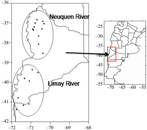
Figure 1. Stations used in the study.
[7] studied the characteristics of rainfall in the Chaco region of Argentina and detected previous circulation patterns associated with wet summer seasons. Some studies focused on studying the relation with El Niño-Southern Oscillation (ENSO) [8-14]. The aim of this paper is to detect the possible relationships between the accumulated rainfall during rainy season in the Comahue region and both, the ocean and atmospheric circulation patterns, previously observed. The paper is organized as follows: Section 2 describes the dataset and the methodology; Section 3 presents the SPI features in Limay (LB) and Neuquen (NB) river basins. Section 4 shows the relation between SPI calculated over the period April to September and atmospheric circulation. The association with SST was detailed in Section 5. Section 6 presents the building of regression models to estimate wet and dry events and Section 7 presents the main conclusions.
2. Data and Methodology
The area under study includes two river basins: the Limay river basin (LB) in the south and the Neuquen river basin (NB) in the north (Figure 1). To carry out this study, there were used monthly rainfall data derived from 20 stations at different sources—the National Meteorological Service, the Secretary of Hydrology of Argentina and the Territory Authority of the Limay, Neuquén and Negro river basins and the 1980-2007 record thereof. The period was selected because all the stations have less than 20% of missing monthly rainfall data and their quality has been carefully proved.
Two mean rainfall series were calculated to obtain the average of monthly precipitation of twelve stations in the NB and eight stations in the LB, in order to be representative of the precipitation over each one of the basins (Figure 1). The standardized precipitation index (SPI) was used to quantify the conditions of deficit or excess of precipitation for a six-month interval, which is the period that better works for hydrological matters [15,16], and with the purpose of improving the detection of rainfall excesses and deficits which could have significant consequences for the operation of dams. Computation of the SPI involves fitting a gamma probability density function to a given frequency distribution of six-month precipitation totals for LB and NB [15]. The SPI greater (lower) than zero indicates water excess (deficit). A wet (dry) period is defined as the period during which the SPI is continuously positive (negative). The magnitude of the index allows classifying the six-month accumulated rainfall in categories that go from extreme drought to extreme excess (extremely dry, severe dry, moderate dry, normal, moderate wet, severe wet and extremely wet). SPI series low frequency variability was analyzed using a linear trend method of minimum squares, and statistics significance was tested using a T-Student test.
There are also used monthly sea surface temperatures (SST), 500 HPa (G500), 1000 Hpa (G1000) and 200 Hpa (G200) geopotential heights, zonal (U) and meridional (V) winds at 850 Hpa and precipitable water (PW) from National Center of Environmental Prediction (NCEP) reanalysis [17]. Monthly anomalies were determined removing the climatologically monthly means from the original values. Composite fields of these variables for wet and dry years and the difference between them are plotted. The statistical significance is checked using a Student’s t-test (95% confidence level) on the difference between the wet and dry means. These significant areas are used to find the existing relation between SPI calculated with accumulated rainfall from April until September (SPI9) in LB and SST, G1000, G500, G200, U and V during the same period and only in April. The results permit to define some predictors, which are used to develop a statistical forecast model using the forward stepwise regression method [18] which retained only the variables correlated with a 95% significance level. Forward stepwise regression is a model-building technique that finds subsets of predictor variables that most adequately predict responses on a dependent variable by linear regression, given the specified criteria for adequacy of model fit [19]. Predictors available to carry out the regression scheme are carefully selected, based on statistical significance and physical reasoning. A polynomial model is also derived using a standard regression method.
The skill of the schemes was proved using contingency tables and a Chi-square test was applied to detect if they differ significantly from random ones. Some measures of accuracy [18] were calculated for wet and dry cases. The hit rate (H) or the right proportion is the fraction of all the cases when the categorical forecast correctly anticipated the subsequent event. The probability of detection (POD) is defined as the fraction of those occasions when the forecast event occurred on which it was also forecast. The false alarm relation (FAR) is the proportion of forecast events that fail to happen. Additionally, empirical estimated and observed SPI9 probability functions were calculated using frequency distributions and a chi-square test was used to prove that they do not differ significantly.
3. SPI Features in LB and NB
Figure 2 shows the six-months SPI for LB and NB series and their respective linear trend adjustment. It is notable that there is no trend in both cases. The duration of each period is defined as the number of months that the SPI retains the same sign and the intensity is the mean SPI over each period. Thirty wet and thirty dry periods were detected in SPI series in LB. Table 1 shows that 53% of the wet periods persists less than 3 months and 23% more than 10 months, meanwhile 60% of dry periods lasts less than 3 months and only 3% lasts more than 10 months, indicating that most of the dry periods are short. Table 2 shows the number, mean duration and mean intensity of wet and dry periods in the sub-periods 1980- 1988; 1989-1997 and 1998-2006. Wet and dry periods during 2007 are disregarded (only in this table) in order for the 3 periods to have the same length. It can be seen that the number of wet periods in LB slightly increases and their duration is shorter and the number of dry periods increases but their intensity and duration remain similar. This result indicates an increase of rainfall variability over time.
Twenty-four wet and twenty-four dry periods are detected in SPI series in NB. Table 1 shows that 37.5% of wet periods lasts more than 10 months and 29% less than 3 months meanwhile most of dry periods are shorter (less
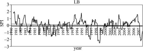
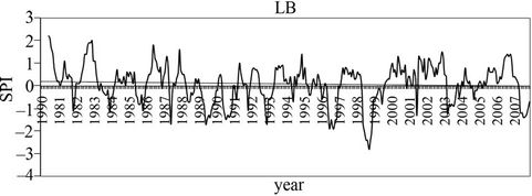
Figure 2. Twelve months SPI for Limay River Basin (upper pannel) and Neuquen River Basin (bottom pannel).
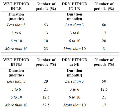
Table 1. Percentage of wet and dry periods with different duration for LB (upper panel) and NB (bottom panel).

Table 2. Number, mean intensity and mean duration of wet and dry periods in 1980-1988, 1989-1997 and 1998-2006 in LB (upper panel) and NB (bottom panel).
than 3 months). Table 2 reveals that there is no specific trend when different time periods are considered.
It is important to notice that there is a tendency for wet (dry) periods to take place in El Niño (La Niña) years in both basins. In fact, in four wet periods in LB—out of the nine wettest ones—the warm phase on ENSO was in its mature stage, meanwhile in two of them La Niña event was developing. But in three dry periods—out of the eight driest ones—La Niña event was present and in two dry periods El Niño events developed. The signal is clearer in NB where, in five—out of the six wettest periods—El Niño was present and La Niña developed in none of them and in three—out of the six driest periods—La Niña was present and El Niño developed in none of them. Therefore, the correlation between sixmonth SPI and SST in EN34 region in the last month of the period is 0.38 in LB and 0.37 in NB, both significant at the 95% confidence level. This particular relation will be described in detail in Section 5.
Figure 3 shows the mean (1980-2007) monthly rainfall in both basins. It reveals that precipitation has an important annual cycle with a maximum in winter. As the most important quantity rainfall amount occurs from April to September, the analysis of SPI9 (SPI for the precipitation accumulated in this period) will be detailed hereinafter. Results in LB and NB were similar but only LB ones will be presented in this paper.
The percentage frequency of SPI9, a summary of the definitions and the years when the different categories took place are presented in Table 3.
4. Relation between SPI9 and the Atmospheric Circulation
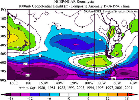
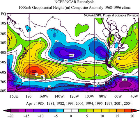
Figure 4 shows the G1000 anomaly composite fields for wet and dry cases during the period April-September and the difference between wet and dry composites, and Figure 5 shows the same only for April. The most important feature is the dipole between high and middle latitudes (Figure 4). In dry composites the subtropical heights and the sub-polar lows are intensified and the subtropical heights extend towards Argentina. Meanwhile, in wet cases both belts are weakened. This pattern remains when composites in April are considered (Figure 5). This is a relevant result because the April geopotential height field could be used for predicting purposes. The same pattern is observed in the composites for each one of individual months in the period May-September (figures not shown). It is important to notice that precipitation systems usually displace over the Pacific Ocean, arrive in the South American coast and can go through the southern portion of the Andes mountains (south of 38˚S), because the latter are lower than in the north. Therefore
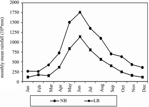
Figure 3. Mean annual cycle of rainfall in NB and LB.
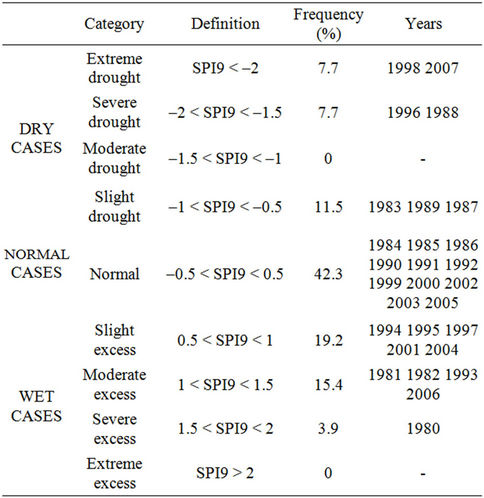
Table 3. Percentage frequency of SPI9, a summary of the definitions and the years when the different categories took place in LB.
the long-lasting weakness of the high pressure belt in wet cases all over the whole period allows cold fronts to intensify and displace more frequently over the basin, thus generating precipitation. This pattern is also observed in G500 and G200 although the center of maximum weakness of subtropical height is slightly displaced (figures not shown).
The same procedure is applied to U and V anomaly composite fields for the April-September period and for April alone. According to the geopotential height pattern, an intensification (weaken) of westerlies is observed in dry (wet) cases in the central and east Pacific Ocean in U and V difference composites (figures not shown). North wind is more frequent than south wind in the Comahue region and there is a tendency that northern winds weaken (intensify) in dry (wet) cases over the basin, as it is revealed in the V anomaly composite fields for the AprilSeptember period and for April alone (figure not shown).
In addition, wet (dry) cases tend to occur when a positive (negative) anomaly of PW is present over central Argentina including LB, and this happens during the whole April-September period and April only (figures not shown).
5. Relation between SPI9 and Sea Surface Temperature
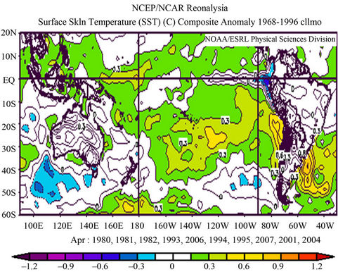
The composites of SST anomaly in wet and dry cases and the difference between them for the period AprilSeptember are detailed in Figure 6. There are evidences that wet (dry) cases tend to occur in warm (cold) phase of ENSO, El Niño (La Niña). The signal is not strong but significant. Another area with important difference of SST between wet and dry cases—although it is not statistically significant—is located in the central Pacific and
 (a)
(a)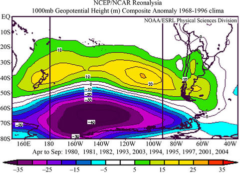 (b)
(b)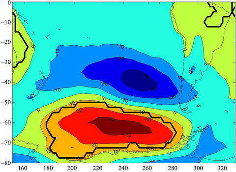 (c)
(c)
Figure 4. Composite of mean 1000 Hpa geopotential heights field since April to September for wet cases (a), dry cases (b) and the difference between wet and dry cases. 95% significant difference in draw in black line [21] .
 (a)
(a)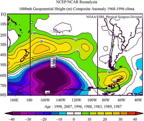 (b)
(b)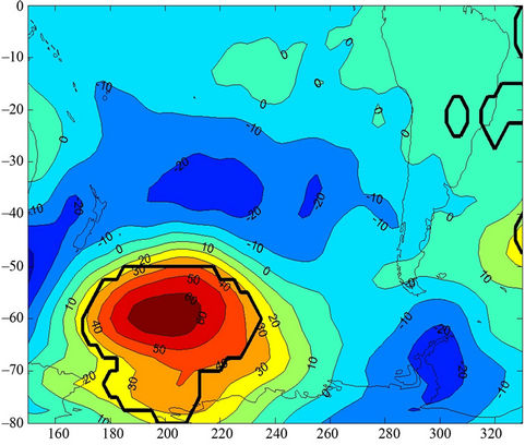 (c)
(c)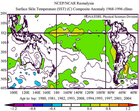 (a)
(a)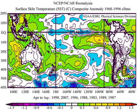 (b)
(b)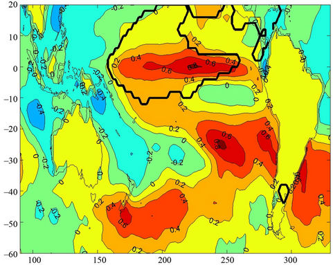 (c)
(c)
Figure 6. Composite of mean SST field since April to September for wet cases (a), dry cases (b) and the difference between wet and dry cases. 95% significant difference in draw in black line [21].
seems to be related to the Rossby wave propagation [20]. When April composites are considered (Figure 7) the
 (a)
(a)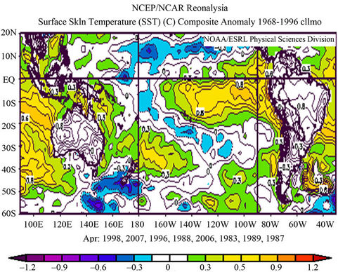 (b)
(b)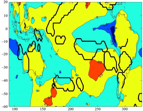 (c)
(c)ENSO signal weakens and concentrates only in the western part of tropical Pacific Ocean. The significance is not high.
6. The Statistical Prediction Model for SPI9
The first stage of the model is to determine predictors that represent the statistical associations between SPI9 and circulation or SST patterns, in order to identify the key elements of the atmospheric circulation that promote or inhibit rainfall anomalies in the study region. It is important to point out that they are carefully selected, taking into account their physical reasoning. Some predictors are defined as the mean value in a given area using the zones with significant differences between wet and dry cases in April (Table 4). The correlation between the defined predictors and SPI9 is calculated and because of the 1980-2007 record, values greater than 0.37 are statistically significant (95% significance level). The bi-serial correlation coefficient [22] is a special case in which one variable is quantitative (the predictor) and the other variable is dichotomous (wet, SPI9 > 0 or dry cases, SPI9 < 0) and nominal. The calculations have typically simplified since the values 1 (wet) and 0 (dry) are used for the dichotomous variable. It represents the ability of the predictor to distinguish wet from dry cases. G10A, G5A and G2A (G10B, G5B and G2B) are the predictors over the areas where the maximum difference between wet and dry cases is detected in the subtropical height (subpolar low) belt. The difference between them are defined (G10D, G5D and G2D), and these predictors result the most relevant ones because of their high correlation with SPI9 (Table 4). That is the reason why they are used to be included in a forward stepwise regression model which will predict SPI9.
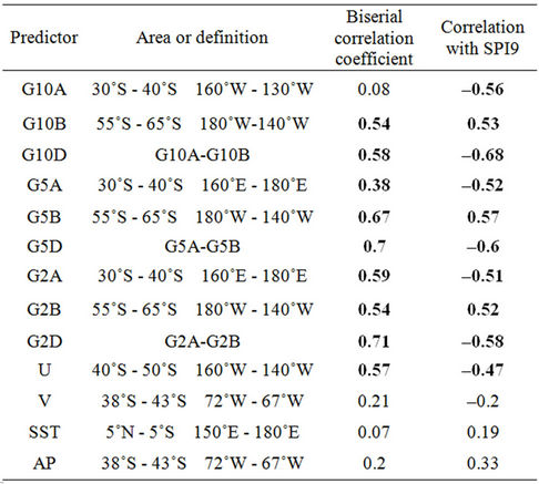
Table 4. Definition of predictors and their correlations with SPI9 and the bi-serial coefficient. Values in italics and bold are significant at the 95% confidence level.
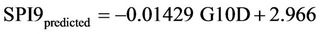
The forward stepwise method selects only G10D as the main predictor and the equation derived from the linear regression forecast model is:
 (1)
(1)
G10D is expressed in m. This model shows the influence of the behavior of low level precipitation systems displacing over the Pacific Ocean on the rainfall in LB. The regression model explained the 46% of the SPI9 variance. A measure of strength of the regression is the F-ratio, defined as the relation between the mean square regression and the mean square error [18]. It is worth pointing out that the F-ratio was high because a strong relation between SPI9 and the predictors will produce large mean square regression and small mean square error. As the residuals of the regression are independent and follow a normal distribution, under the null hypothesis of no lineal regression, the F-ratio is 22.1 with a p-value of 0.00007, indicating that the regression model provides reasonably forecast with 95% of confidence. A cross-validation method is applied in which out of 28 years, 27 are used for calibration and the process are repeated 28 times. This approach is useful when the dataset is relatively short and it is more robust in the presence of a long-term climate variability, which should show up as a gradual drift in the regression parameters. As three predictors entered the model and the model is constructed for 28 years, there was no case of overfitting; and as the model remains similar, there is evidence of numerical stability. Figure 8 shows the observed and predicted SPI9 which present a correlation coefficient between them of 0.61. In Figure 8 the largest discrepancy between predicted and observed SPI9 is produced in the years 1990, 1994, 2000, 2001 and 2004 and none of which has been an extreme drought or excess. Considering excess (drought) cases when SPI9 is greater (less) than zero, some efficiency measures are calculated and the following values are derived: POD 59%, FAR 29% and H 75%. In order to convert the individual estimations in a probabilistic forecast, the accumulated frequencies are calculated for the observed and forecast SPI9 values and the empiric probability functions are drawn (Figure 9). A chi square test is used and the empiric probability functions are significantly similar at the 95% confidence level.
In order to improve the linear scheme, a polynomialbased non parametric method for forecasting SPI9 is developed using a standard method for predictor G10D (Figure 10). The estimation derived equation is:
 (2)
(2)
It explains the 49% of the variance of SPI9 and F is 12.09 with p of 0.00021. The cross-validation scheme produces an estimated series which is significant correlated (0.62) with the observed one. The values of efficiency

Figure 8. Observerd and predicted SPI9 using a multiple linear regression model. The model is SPI9predicted = –0.01429 G10D + 2.966 and R is 0.68.
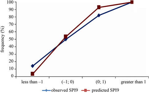
Figure 9. Empiric probability functions for observed and predicted SPI9.
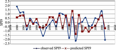
Figure 10. Observerd and predicted SPI9 using a polynoal regression model. The model is: SPI9predicted = 0.0185 G10D – 0.000083 G10D2 – 0.0924 and R is 0.7.
statistics are: POD 71%, FAR 29% and H 71%. The conclusion is that the polynomial method does not improve the linear one to a great extent.
7. Conclusions
In this paper the area under study includes two basins: the Limay and the Neuquen river basins, both relevant because of the hydroelectric dams which are on these rivers. Rainfall accumulated during the rainy season (since April to September), represented by SPI9, was particularly studied for LB. The main goal of this work is to detect previous (April) circulation and oceanic patterns which could be used as predictors for a possible extreme rainy season. Moreover an approach to estimate quantitative value of SPI9 was developed. Although there is a tendency for wet (dry) periods to take place in El Niño (La Niña) years, the statistical linear model proved that the main factor which influenced rainfall was the behavior of low level precipitation systems displacing over the Pacific Ocean. The linear model resulted efficient in forecasting SPI9 and its greatest failures occurred in non-extreme years. The polynomial model improved less than the linear one. The application of these results improves the efficiency in dam operation, thus producing a more sustainable energy generation.
8. Acknowledgements
Rainfall data were provided by the National Meteorological Service, the Secretary of Hydrology of Argentina and the territory Authority of the Limay, Neuquén and Negro river basins. Images from Figures 4, 7(a) and (b) were provided by the NOAA/ESRL Physical Sciences Division, Boulder Colorado from their web site: http:// ww.dc.noaa.gov [22]. This research was supported by UBACyT 2010-2012 CC02, UBACyT 2011-2014 1028, PICT BICENTENARIO 2010-2110 and CONICET PIP 112-200801-00195.
REFERENCES
- T. Gissila, E. Black, D. I. F. Grime and J. M. Slingo, “Seasonal Forecasting of the Ethiopian Summer Rains,” International Journal of Climatology, Vol. 24, No. 11, 2004, pp. 1345-1358. doi:10.1002/joc.1078
- C. Reason, “Subtropical Indian Ocean SST Dipole Events and Southern Africa Rainfall,” Geophysical Research Letters, Vol. 28, No. 11, 2001, pp. 2225-2227. doi:10.1029/2000GL012735
- X. Zheng and C. Frederiksen, “A Study of Predictable Patterns for Seasonal Forecasting of New Zealand Rainfall,” Journal of Climate, Vol. 19, No. 13, 2006, pp. 3320-3333. doi:10.1175/JCLI3798.1
- M. H. González and C. S. Vera, “On the Interannual Winter Rainfall Variability in Southern Andes,” International Journal of Climatology, Vol. 30, No. 5, 2010, pp. 643-657
- M. H. González, M. M. Skansi and F. Losano, “A Statistical Study of Seasonal Winter Rainfall Prediction in the Comahue Region (Argentine),” Atmosfera, Vol. 23, No. 3, 2010, pp. 277-294.
- M. L. Cariaga and M. H. González, “Estimating Winter and Spring Rainfall in the Comahue Region (Argentine) Using Statistical Techniques,” Advances in Environmental Research 11, Justin A. Daniels, Nova Science Publishers Inc., New York, 2011, pp. 103-128.
- M. H. González and A. M. Murgida, “Seasonal Summer Rainfall Prediction in Bermejo River Basin in Argentina,” Climate Variability, Abdel Hannachi, Intech, Reading, 2011, in Press.
- C. Schneider and D. Gies, “Effects of El Niño-Southern Oscillation on Southernmost South America Precipitation at 53˚S Revealed from NCEP-NCAR Reanalysis and Weather Station Data,” International Journal of Climatology, Vol. 24, No. 9, 2004, pp. 1057-1076. doi:10.1002/joc.1057
- P. Aceituno, “On the Functioning of the Southern Oscillation in the South American Sector. Part I: Surface Climate,” Monthly Weather Review, Vol. 116, No. 3, 1988, pp. 505-524. doi:10.1175/1520-0493(1988)116<0505:OTFOTS>2.0.CO;2
- P. Aceituno and R. Garreaud, “Impactos de Los Fenó- menos El Niño y La Niña Sobre Regímenes Fluviométricos Andinos,” Revista de la Sociedad Chilena de Ingeniería Hidráulica, Vol. 10, No. 2, 1995, pp. 33-43.
- J. Rutland and H. Fuenzalida, “Synoptic Aspects of the Central Chile Rainfall Variability Associated with the Southern Oscillation,” International Journal of Climatology, Vol. 11, No. 1, 1991, pp. 63-76. doi:10.1002/joc.3370110105
- P. Aceituno, “Seasonality of the ENSO Related Rainfall Variability in Central Chile and Associated Circulation Anomalies,” Journal of Climate, Vol. 16, No. 2, 2003, pp. 281-296. doi:10.1175/1520-0442(2003)016<0281:SOTERR>2.0.CO;2
- R. Compagnucci and W. Vargas, “Inter-Annual Variability of the Cuyo River Streamflowin the Argentinean Andean Mountains and ENSO Events,” International Journal of Climatology, Vol. 18, No. 14, 1998, pp. 1593-1609. doi:10.1002/(SICI)1097-0088(19981130)18:14<1593::AID-JOC327>3.0.CO;2-U
- R. Compagnucci and D. Araneo, “Identificación de Áreas de Homogeneidad Estadística Para los Caudales de los Ríos Andinos Argentinos y su Relación Con la Circulación Atmosférica y la Temperatura Superficial del Mar,” Meteorologica, Vol. 30, No. 1, 2005, pp. 41-54.
- T. B. Mckee, N. Doesken and J. Kleist, “The Relationship of Drought Frequency and Duration to Times Scales,” Proceeding 8th Conference of Applied Climatology, Anaheim, 17-22 January 1993.
- T. B. McKee, N. Doesken and J. Kleist, “Drought Monitoring with Multiple Time Scales,” Proceeding 9th Conference on Applied Climatology, Dallas, 15-20 January 1995.
- E. Kalnay, M. Kanamitsu, R. Kistler, W. Collins, D. Deaven, L. Gandin, M. Iredell, S. Saha, G. White, J. Woollen, I. Zhu, M. Chelliah, W. Ebisuzaki, W. Higgings, J. Janowiak, K. C. Mo, C. Ropelewski, J. Wang, A. Leetmaa, R. Reynolds, R. Jenne and D. Joseph, “The NCEP/ NCAR Reanalysis 40 Years-Project,” Bulletin of the American Meteorological Society, Vol. 77, 1996, pp. 437-471. doi:10.1175/1520-0477(1996)077<0437:TNYRP>2.0.CO;2
- D. S. Wilks, “Statistical Methods in the Atmospheric Sciences (An Introduction),” International Geophysics Series Academic Press, San Diego, 1995.
- R. B. Darlington, “Regression and Linear Models,” McGrawHill, New York, 1990.
- E. Kalnay, K. C. Mo and J. Paegle, “Large-Amplitude, Short Scale Stationary Rossby Waves in the Southern Hemisphere: Observations and Mechanistics Experiments on Determine Their Origin,” Journal of the Atmospheric Sciences, Vol. 43, No. 3, 1986, pp. 252-275. doi:10.1175/1520-0469(1986)043<0252:LASSSR>2.0.CO;2
- NOAA/ESRL Physical Sciences Division, Boulder Colorado, 2011. http://www.cdc.noaa.gov
- H. Panofsky and G. Brier, “Some Applications of Statistics to Meteorology,” The Pennsylvania State University, Pennsylvania, 1965.