International Journal of Astronomy and Astrophysics
Vol.1 No.3(2011), Article ID:7365,8 pages DOI:10.4236/ijaa.2011.13019
Observational Evidences for Extremely Strong Magnetic Fields in Solar Flares
Kyiv University Astronomical Observatory, Kyiv, Ukraine
E-mail: lozitsky@observ.univ.kiev.ua
Received July 5, 2011; revised August 10, 2011; accepted August 20, 2011
Keywords: Sun, Solar Flares, Small-Scale Magnetic Fields, Superstrong Fields
Abstract
New observational data related to the X1.1/2N solar flare of 17 July 2004 were investigated and compared with some old data for other powerful flares and non-flare regions. Observations were carried out with the Echelle spectrograph of the Kyiv University Astronomical Observatory. The Stokes I ± V profiles of several metallic lines with different effective Lande factors geff have been analyzed including the FeI 5434.5 line with very low magnetic sensitivity (geff = –0.014). The obvious evidences of the emissive Zeeman effect were found as in lines with great and middle Lande factors as in FeI 5434.5 line. On the basis of all analyzed data one can conclude that upper magnetic field limit in flares can reach 70 - 90 kG, i.e. about more order higher than the well-known magnetic fields in great sunspots. The possible physical nature of such superstrong fields is discussed.
1. Introduction
The upper magnetic field strength limit in the solar atmosphere is unknown at present. The point of view predominates that the strongest fields exist at great sunspots. Parker [1] said: “More recently we have come to appreciate that the sunspots is just the most conspicuous feature of a vast word of magnetic activity”. According to observations, the field strength is here, as rule, 2100 - 2900 G and sometime 3500 - 4000 G. The record field of 6100 G in a sunspot was measured by Livingston et al. [2].
Solar flares are very interesting and violent processes in solar active regions where the strongest fields could exist too. Each flare is a grandiose explosion in a wide range of height in solar atmosphere, with sharp increaseing of temperature, gas pressure and ionization of plasma. Hot flare plasma outside magnetic flux tubes should press on walls of these tubes and may increase magnetic strength inside tubes. In addition, increasing of plasma ionization leads to amplification of electric currents and to magnetic field intensification, if structure of magnetic field is force-free.
Unfortunately, magnetic field measurements in flares are not quite simple as in sunspots. First of all, solar flares occur suddenly and develop rapidly. The most interesting phases of a flare can be missed if observations carry out in non-continuous regime. Namely such noncontinuous regime is usual for spectral observations, but namely spectral observations are the most suitable for magnetic field measurements in flares. As to instruments working in automatic regime like SOHO/MDI filter magnetograph, ones give mainly longitudinal magnetic field component—no field module. In addition, in case of the most powerful flares practically all spectral lines have more or less intensive flare emission. In some cases, this emission distorts magnetographic signal sufficiently and leads to the false field values, even false measured polarity [3-5].
As to spectral observations, some authors assumed the upper magnetic field strength limit in range of 50 - 100 kG [6,7]. In particular, Severny [6] assumed the 50 kG fields in small-scale (spatially unresolved) magnetic elements of sunspots. He wrote: “Thus, it is quite possible, that magnetic field inside sunspots has a fine structure, which is averaged during the observations and gives the fields of 103 gauss, whereas the true field in the separate elements of sunspots (perhaps, of different magnetic polarity and inclination) reachs of several tens of kilo-gauss; i.e. situation can be the same as in a case of granulation where the averaging of separate fields of granules (~100 gauss) leads to measured field on level of a few gauss”.
Bruce [7] supposed that long wings of Hα line in flares (till 8 Å) could arise due to the Zeeman effect in 10 - 100 kG fields. Really, this is one of possible interpretation: some account to the line-profile broadening should give also temperature, turbulent velocity and electric fields. For these effects separation, the full Stokes parameters I, Q, U and V of polarized light are needed. In other hand, if magnetic field is subtelescopically tangled (for instance, in form of mixed polarity structures) the Stokes diagnostics could be useless: we can have essential broadening of Stokes I profile but practically zero polarization on different distances from line center.
More direct evidences to such “superstrong” fields in flares were obtained using observations in FeI lines with very low Lande factors [8-11]. It was shown that Stokes I ± V profiles of some such lines, e.g. FeI 5F15F1 λ = 5123.723 Å and FeI 5F15D0 λ = 5434.527 Å, have in flares narrow and splitted emission peaks in their cores. Both named lines have the following Lande factors: theoretically, for LS coupling, gLS = 0.000, but laboratory determined values gLab = –0.013 and –0.014, respectively [12,13]. Observed splitting of emission peaks in I ± V profiles was ΔλV = 10 – 36 mÅ, whereas similar splitting in I ± Q profiles was close to zero (ΔλQ ≤ 5 mÅ). Taking into account that non-flare profiles did not display similar effects, it was assumed the Zeeman effect manifestation in field of B ≈ 26 - 94 kG.
Naturally, such extraordinary conclusion needs an additional and careful verification on a base of new data for other flares. Unfortunately, this is almost insuperable task for spectral observations. Enough bright flare emismsion in FeI 5123.723 and 5434.527 cores occur in very powerful solar flares only, of X1 class or more. More weak flares, e.g. of M or C importance, produce, as rule, ordinary Fraunhofer line profiles, without emission peaks in their cores. So, only unique spectral data are suitable to the problem, related to the suddenly occurred large and bright solar flares.
Some of such flares were observed on Echelle spectrograph of horizontal solar telescope of Kyiv University astronomical observatory [14]. About five decades from 1950s, this instrument is used for regularly carried out spectral observations in wide range of wavelength, from 3800 to 6600 Å. Till 1975 these observations were made in Stokes I, but since 1975—in Stokes I ± V and I ± Q too. In this work, the new observational data related to the X1.1 solar flare are presented and analyzed.
2. Observational Data and Profiles of Lines
Flare of 17 July 2004 had occured in active region 10,649, at its tail part placed closely to spots of N polarity with magnetic strength of 2800 G and heliocentric distance μ = 0.88. Observations of the flare were carried out with the Echelle spectrograph of the Kyiv University Astronomical Observatory [14]. From 8:01 to 8: 16 UT six Echelle Zeeman spectrograms were obtained with a circular polarization analyzer, but at present study the first spectrogram only is analyzed containing the strongest flare emission (Figure 1), nearest to time of the X ray peak according to GOES data (7:56 UT). All
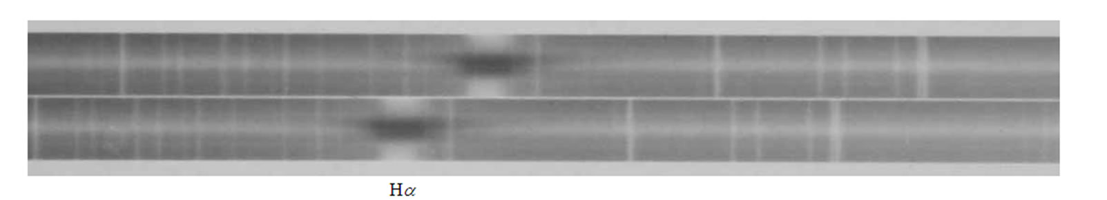
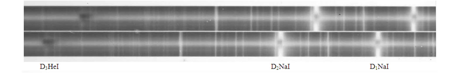
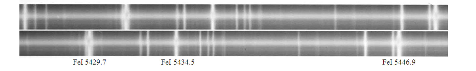
Figure 1. Fragments of the Echelle Zeeman spectrogram (I + V and I – V spectra) showing the flare emission (for 8:01 UT) in some spectral lines.
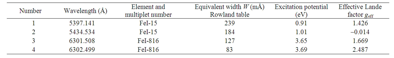
Table 1. List of selected spectral lines.
spectra were made with ORWO WP3 photoemulsion.
Four spectral lines of FeI were used for magnetic field measurements in area of flare—two lines of 15th multiplet and two lines of multilplet No. 816 (Table 1). Lines Nos. 3 and 4 form at level of middle photosphere whereas the cores of lines Nos. 1 and 2—in range of upper photosphere and temperature minimum zone. Effective Lande factors geff listed in the table correspond to laboratory determined values from papers [12,13]. As it was pointed out above, theoretical effective Lande factor for 5434.534 line is geff = 0.000 for case of LS coupling. At first approximation, this line can be considered as Doppler one, whereas other three lines—as Zeeman sensitive lines. Only in case of very strong fields of ~104 G range, FeI 5434.5 should be considered as Zeeman line too [8].
Photometrical study with microphotometer MF-4 shown that lines Nos. 3 and 4 have ordinary Fraunhofer profiles in the flare, without any emission peaks at their cores (Figure 2). On this figure, Δλ is distance (in mÅ) from center of telluric line O2 λ = 6302.000 Å. Centers of lines FeI 6301.5 and FeI 6302.5 correspond to Δλ about –500 and +500 mÅ, respectively; second telluric line O2 has Δλ ≈ 750 mÅ. Three photometrical sections Nos. –19, –21 and
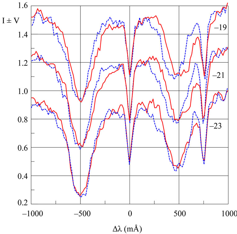
Figure 2. Observed Stokes I ± V profiles for the FeI 6301.5 and 6302.5 lines in the flare (see text).
–23 related to strongest flare emission are presented here. Space interval between nearest sections (e.g. –19 and –21) corresponds to 1 Mm on the Sun. Distribution of intensity for section No.–23 is original, whereas other distributions are shifted along ordinat axis on 0.3 and 0.6 in unit of continuum level.
One can see the lack of full Zeeman splitting in FeI 6302.5 line with the highest magnetic sensitivity (geff = 2.487) that indicates the moderate longitudinal magnetic field—of subkilogauss range (<1 kG). The FeI 5397.1 line has more complicated and interesting profiles—with Fraunhofer wings and emission peaks in line core (Figure 3).
Second interesting effect: splitting of emission peaks appreciably exceeds the splitting of line wings. Similar effect for flares was found earlier by Lozitska and Lozitsky [3]. Notice, emission peaks in lines like FeI 5397.1 form at upper photosphere whereas Fraunhofer wings—below named level [15]. Thus, this second effect is evidence to the local magnetic field amplification at some level of the flare.
3. Measured Magnetic Fields
Magnetic fields in area of the flare were measured using
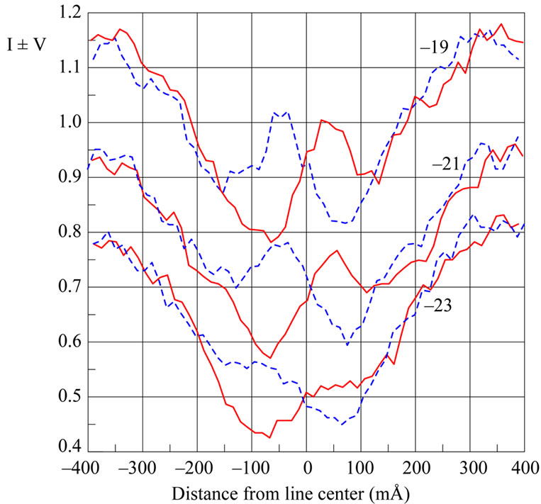
Figure 3. Observed Stokes I ± V profiles for the FeI 5397.1 line in the flare.
two methods: a) by splitting of “center of gravity” of whole I ± V profiles and b) by relative shifts of limited intervals of these profiles. In first method, relative shift of the 'centers of gravity' of the I + V and I – V profiles is interpreted as a result of the Zeeman Effect and calibrated in values of magnetic field using well known formula
 (1)
(1)
where the Zeeman splitting DlH and wavelength l are in Å, and field strength B in gauss (G). In a case of homogeneous field and small Zeeman splitting (exactly, if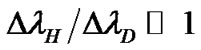 , where DlD is the Doppler half width of line), the longitudinal magnetic component B║ can be obtained from such measurements. If magnetic field is inhomogeneous, such observations give likely the longitudinal magnetic flux [16].
Measurements with second method were calibrated analogously, using formula (1) too. For the same spectral line, these data reflect the magnetic field strength in narrower interval of height in solar atmosphere than ‘center of gravity’ data. It is useful to remember, that second method is similar methodically to classical magnetographic measurements [17] with fixed exit slits in line profile.
First method was applied to FeI 6301.5 and 6302.6 lines, and second—to FeI 5397.1 (Table 2). In this table, measurements in FeI 5397.1 for |Δλ| = 200 – 300 mÅ correspond to Fraunhofer wings of line, and for |Δλ| = 0 – 200 mÅ—to splitted emission peaks in line core. The error bars are about ±40 G for FeI 6302.5, ±60 G for FeI 6301.5 and ±75 G for 5397.1. One can see that all three magnetosensitive lines (excluding FeI 5397.1 for |Δλ| = 0 – 200 mÅ) give similar results. In photometrical section No.–23 (which places closely to magnetic inversion line B║ ≈ 0) all lines give practically coincided results, whereas in sections Nos. –19 and –21 the measured field strengths are some differ. At these sections, the following inequality is obvious: B5397.1 < B6301.5 < B6302.5. Taking into account that equivalent widths of lines W correlate as: W5397.1 > W6301.5 > W6302.5, we can admit the negative vertical magnetic field gradient ( ) at photospheric layers of the flare.
Likely, such situation (i.e.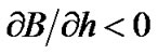 ) was in a limited range of photosphere. As it follows from splitting of

Table 2. Comparison of the magnetic fields measured in different lines and places of the flare.
emission peaks of FeI 5397.1 line (Δλ = 0 – 200 mÅ), the kilogauss fields (B ≈ 2.1 – 2.9 kG) had existed in upper photoshere. Thus, we can expect that at lest two layers were in area of flare: a)  in range of the middle photosphere, and b)
 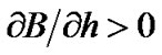 at upper level. Perhaps this indicates non-monotonous magnetic field distribution in area of the flare similar to a case described earlier by Lozitsky et al. [15] for another flare.
4. Polarized Effects in Core of FeI 5434.5 Line
Observed I ± V profiles of FeI 5434.5 line in flare of 17 July 2004 are presented on Figure 4. Similar to cases of FeI 6301.5, 6302.6 and FeI 5397.1 lines (see above Figures 2 and 3), distribution of intensity for section No.–23 is original, whereas other distributions are shifted along ordinat axis on 0.3 and 0.6 in unit of continuum level.
One can see the following:
1) Fraunhofer wings (|Δλ| > 100 mÅ) and narrow emission peaks in line core (|Δλ| < 100 mÅ); observed half-widths of these peaks are very small, about 50 mÅ;
2) Fraunhofer wings of I + V and I – V profiles are, in general, in good agreement—differences between these profiles are, as rule, less than 1%;
3) Differences between I + V and I – V profiles in line core are larger and reach 3% - 4%; this means presence of weak circular polarization here;
4) Locations of emission peaks in I + V and I – V profiles coincide, in general, in photometrical section No. –19, but ones are some different in sections Nos. –21 and
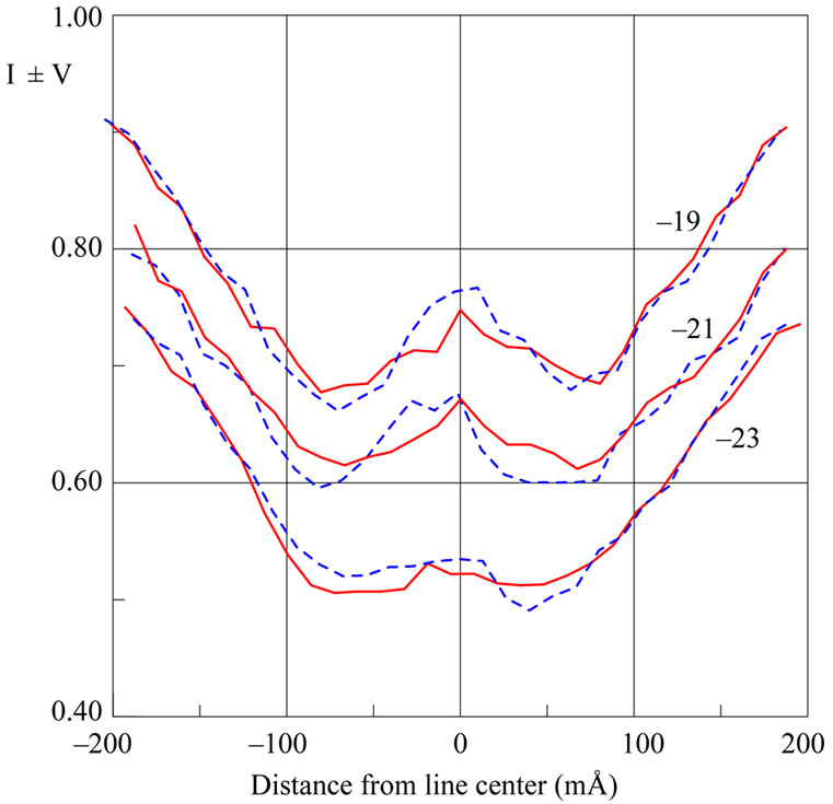
Figure 4. Observed Stokes I ± V profiles of FeI 5434.5 line in flare of 17 July 2004.
–23. At two last sections, pictures of I ± V profiles at their central parts looks as spectral splitting of tops of emission peaks. Value of this splitting reaches about 30 mÅ.
For estimation of noise level and possible error bars, similar photometrical I ± V profiles are needed observed in non-flare area too. Another way is suitable to this task: study of similar profiles of any strong telluric line; such line, naturally, should be considered as pure non-magnetic one.
For this purpose, FeI 5434.5 line was studied outside the flare—in area of weak magnetic field (B║ < 100 G). In addition, non-magnetic effects were estimated by telluric H2O λ = 5919.644 Å line observed on very large air mass, M = 21.2 (Figure 5).
From Figure 5 follows that observed line profiles outside flare are smooth, with small (less than 1% - 2%) differences between I + V and I – V profiles. From this point of view, observed effects in the flare reaching of 3% - 4% (Figure 3) likely are real.
5. FeI 5434.5 Line in Other Flares (Old Data)
Firstly similar features in core of FeI 5434.5 like Zeeman Effect were discovered in 2B-flare of 16 June 1989 [8]. Later, such spectral manifestations were found also in FeI 5123.7 line with effective Lande factor gLab = –0.013 [9]. Lozitsky and Staude [10] observed weak splitting of bisectors of I + V and I – V profiles in core of FeI 5576.1 line (gLab = –0.012) in solar flare of 5 November 2004; if this splitting to interpret as Zeeman effect, corresponding magnetic field is 10 - 15 kG. So, spectral features like Zee-
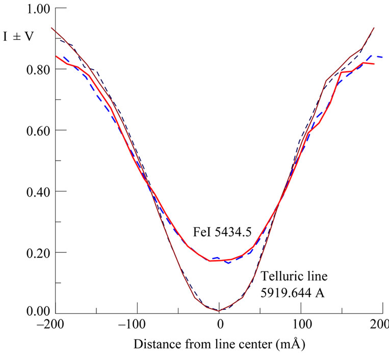
Figure 5. Observed Stokes I ± V profiles of FeI 5434.5 line outside flare and telluric line H2O λ = 5919.644 Å (see text).
man effect were found in all three well known “nonmagnetic” lines—FeI 5123.7, 5434.5 and 5576.1.
An example of such manifestations is given on Figure 6 for flare of 16 June 1989 [11]. One can see well visible splitting of emission peaks in core of FeI 5434.5 line; its value is close to 30 mÅ. There is characteristic splitting also bisectors of I + V and I – V profiles (thin lines on Figure 6): they are practically unsplitted in Fraunhofer wings (|Δλ| > 100 mÅ), but essentially splitted ( ≈12 mÅ) —in line core.
Calculations showed [9] that observed I ± V profiles like presented here on Figure 6 can occur owing to multi-component magnetic field structure (Figure 7). Namely, it is possible to present the observed profile as a sum of Fraunhofer profile 1, unpolarized flare emission 2, first polarized emission 3 and second polarized emission 4; summary profile is presented here as 5. Half-width of unpolarized emission is about 55% relatively Fraunhofer profile 1, flare emission 3 – » 40% and flare emission 4% - 20% only. Magnetic fields was assumed zero for unpolaried emission, 3.5 kG and 65 kG for first and second polarized emission, respectively.
So, these calculations can reflect the following interesting effect: half-width of line profiles are the less, the more is magnetic field strength in subtelescopic fine structures. Earlier narrow spectral lines (» 30% - 50% in unit of undisturbed profile) in subtelescopic magnetic elements with strong field were assumed by Lozitsky [18] and also Lozitsky and Tsap [19] on a base of non-flare magnetic field observations.
Naturally, calculated line profiles presented on Figure
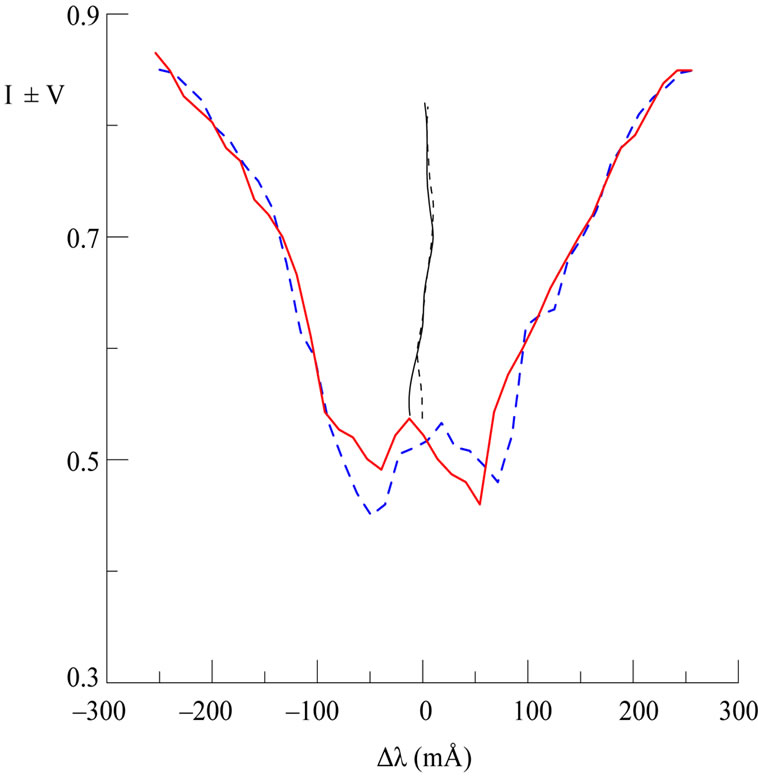
Figure 6. Observed Stokes I ± V profiles of FeI 5434.5 in solar flare of 16 June 1989 (Lozitsky, 2009).
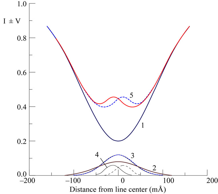
Figure 7. Calculated I ± V profiles of FeI 5434.5 line (see text).
7 are very idealized—they do not present all fine details of observed profiles (Figure 6). Some of these details could have instrumental nature, but other—solar one. More detailed study shown that three types of the Zeeman-like perturbation occur in core of FeI 5434.5 line in area of solar flares [9]:
1) NE (“normal Zeeman”) type has appreciable relative shift of emission peaks in line core, but good agreement of I ± V profiles in line wings; namely such effect is presented on Figure 6 in line core, |Δλ| < 100 mÅ ;
2) CE (“crossover-emission”) type has one-peak emission in I + V profile (or I – V), but two-peak emission in I – V (or I + V); one can see similar picture on Figure 4 for photometrical sections No. –21. In the majority of cases, one-peak emission places in the middle position between two-peak one;
3) A (“absorption”) type is observed in Fraunhofer profiles at their central parts; such effect one can see from bisectors splitting on Figure 6. Similar features were observed also in pure Fraunhofer profiles outside flares.
In favour of Zeeman nature of named effects indicate also observations of I ± Q profiles of FeI 5434.5 line [9]. It was shown that profiles I + Q well coincide with I – Q (in the same positions of flares) and did not display any trustworthy (more than 3 mÅ) splitting of emission peaks in line core.
Preliminary statistics of NE effect is given on Figure 8 [9]. On this histogram, DlB* is splitting of emission peaks in line core relatively line wings. It was assumed that DlB* > 0, if sign of emission peaks is the same as for other magnetosensitive lines with geff > 0, and DlB* < 0 in the opposite case. One can see that distribution for
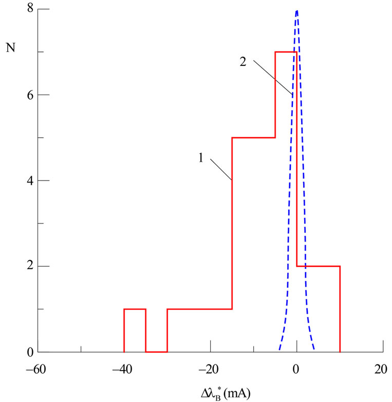
Figure 8. Distrubution of splitting DlB* in core of FeI 5434.5 line observed in flares (1) and non-flare region (2) according to [9]; N—number of cases.
flares (1) is much wider than for a non-flare region (2). In first approximation, distribution (2) can be considered as instrumental, caused by noise fluctuations on spectrograms. Majority of these flustuations are less than 3 mÅ, whereas the values of DlB* for flares (1) are much wide—in range from –40 mÅ to +10 mÅ.
Second important peculiarity: cases of DlB* < 0 for flares (1) predominate over DlB* > 0. This means that our observations confirm the negative sign of effective Lande factor of FeI 5434.5 line (remember, it is –0.014). But, naturally, such “superfine” effect could be discovered only in case if “superstrong” magnetic fields (~104 G) produced the line splitting.
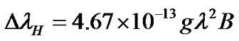
In fact, from formula (1) follows that magnetic field strength B for FeI 5434.5 line can be calculated via
 (2)
(2)
where В is in Gauss (G), and DlН– in Å. If we assume DlB* = 2DlН (really, this is true for longitudinal magnetic field only), then for DlB* = 30 mÅ we have DlН = 15 mÅ, and B » 78 kG. The strongest magnetic fields in flares from distribution (1) reach of B » 90 kG (DlB* = 36 mÅ).
6. Discussion and Conclusion
6.1. Pashen-Back Effect
This effect takes place in strong fields when the following condition is met [20]:
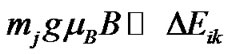 (3)
(3)
where mj is the magnetic quantum number, g is the Lande factor, mB is the Bohr magneton, B is the magnetic field strength, and DEik is the energy difference in the atom between the terms of multiplet structure.
The FeI 5F15D0 λ = 5434.527 Å line belongs to multiplet No. 15 [21]. Its Lande factors for lower (l) and upper (u) terms are following: gl = –0.014, gu = 0/0 that gives for effective Lande factor the above pointed value geff = –0.014. For lower splitted term with excitation potential EP = 1.01 eV, the nearest term is 5F2; it has EP = 0.99 eV and g = 0.5. Then we can assume DEik = 0.02 eV. Substituting ≈ for  in Equation (3) yields an expression to estimate the “threshold” field Bp:
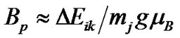 (4)
(4)
Substituting in the numerical values of mj = 2, g = 0.5 and mB = 0.58 ´ 10–8 eV/G, we obtain Bp ≈ 3.4 ´ 106 G = 3.4 MG. Thus, one cannot expect any significant PashenBack effect in case of FeI 5434.5 line for field strength of ~104 G. This means that our application of formula (2) and magnetic field estimations are correct.
6.2. Possible MHD Model
Obviously, such very strong fields can not occur in the simplest case of untwisted magnetic flux tube. In fact, if magnetic flux tube is homogeneous and untwisted, the condition
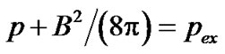 (5)
(5)
should be met, where p and pex are the gas pressures inside and outside the tube, respectively. If we assume pex ~ 104 dyn cm–2 for upper photosphere level where the emission peaks of lines like FeI 5434.5 arise and also p = 0, we obtain B ≈ 500 G only.
More strong fields should exist in twisted force-free magnetic structures. It was shown that a theoretical interpretation of “superstrong” magnetic field phenomena can be offered within the frame of a linear force-free model [22]. This model describes by Bessel’s functions J0 and J1 of zero and first orders; transversal magnetic field distribution is given on Figure 9. This model has a multipolar periphery and magnetic field till ~104 G with discrete values near the tube axis.
From the qualitative point of view, such a multipolar periphery could give a spectral signature similar to a strong ‘mixed polarity’ background field. The theoretical values of discrete strengths near the tube axis are following for photospheric level: 2.5 kG, 6.3 kG, 8.3 kG, 10.0 kG, 11.5 kG, 12.8 kG, etc. Thus, many modes of magnetic field structures can exist for the same gas pressure pex.
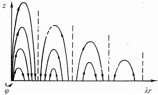
Figure 9. Transversal magnetic field distribution in linear force-free model by Soloviev and Lozitsky [22]. Here z an r are axis and radial coordinates, respectively. Entire lines with arrows indicate magnetic field lines.
However, it is doubtful that this model is suitable for interpretation above-named results with magnetic fields of 70 - 90 kG. The essence of the problem is in necessity of very large number of discrete layers with opposite magnetic polarity inside proper structure. Such layers are marked on Figure 9 via stroke vertical lines. For instance, magnetic field strength of 2.5 kG (see above) can arise in a structure with one layer only. Further, field strength of 6.3 kG needs two layers, field of 8.3 kG - three layers, etc. It is clear, for field of 70 - 90 kG very many discrete layers are needed inside one small-scale (perhaps, subtelescopic) structure! Such many-lamellar magnetic field structure seems as unlikely. In other hand, namely such structures give a strong spectral camouflaging of the superstrong fields if these structures are spatially unresolved: in this case, we should observe essential widening of the magnetosensitive spectral line but practically zero Zeeman polarization at its wings. This assumption agrees with many-component structure of flare emission (see above Figure 7) and with presence of relatively strong unpolarized emission and weak-polarized (i.e. weak-splitted) one.
Naturally, named difficulty of theoretical interpretation does not refute the empirical data partly presented above on Figures 4, 6 and 8. The trustworthy polarized effects were discovered in several solar flares and these effects can not occur in kG fields—they need more strong fields, ~104 G. Probable existence of such superstrong fields presents a very important problem for modern solar physics.
7. References
[1] E. N. Parker, “Solar Activity and Classical Physics,” Chinese Journal on Astronomy and Astrophysics, Vol. 1, No. 2, 2001, pp. 99-124. doi:10.1088/1009-9271/1/2/99
[2] W. Livingston, J. W. Harvey and O. V. Malanushenko, “Sunspots with the Strongest Magnetic Fields,” Solar Physics, Vol. 239, No. 1, 2006, pp. 41-68. doi:10.1007/s11207-006-0265-4
[3] N. I. Lozitska and V. G. Lozitsky, “Do Magnetic Transients Exist in Solar Flares?” Soviet Astronomy Letters, Vol. 8, No. 4, 1982, pp. 270-275.
[4] N. Lozitska and V. Lozitsky, “Small-Scale Magnetic Fluxtube Diagnostics in a Solar Flare,” Solar Physics, Vol.151, No. 2, 1994, pp. 319-331. doi:10.1007/BF00679078
[5] D. N. Rachkovsky, T. T. Tsap and V. G. Lozitsky, “Small-Scale Magnetic Field Diagnostics Outside Sunspots: Comparison of Different Methods,” Journal of Astrophysics and Astronomy, Vol. 26, No. 4, 2005, pp. 435-445. doi:10.1007/BF02702449
[6] A. B. Severny, “Some Results of Investigations of Non-Stationare Processes on the Sun,” Astronomicheskii Zhurnal, Vol. 34, No. 5, 1957, pp. 684-693.
[7] C. E. R. Bruce, “Magnetic Fields in Solar Flares,” Observatory, Vol. 86, No. 951, 1966, pp. 82-83.
[8] V. G. Lozitsky, “Superstrong Magnetic Fields in the Solar Atmosphere,” Kinematics and Physics of Celestial Bodies, Vol. 9, No. 3, 1993, pp. 18-25.
[9] V. G. Lozitsky, “Observations of Magnetic Fields with Strengths of Several Tesla in Solar Flares,” Kinematics and Physics of Celestial Bodies, Vol. 14, No. 5, 1998, pp. 307-316.
[10] V. G. Lozitsky and J. Staude, “Observational Evidences for Multi-Component Magnetic Field Structure in Solar Flares,” Journal of Astrophysics and Astronomy, Vol. 29, No. 3-4, 2008, pp. 387-404. doi:10.1007/s12036-008-0051-9
[11] V. G. Lozitsky, “Observational Evidences to the 105 G Magnetic Fields in Active Regions on the Sun,” Journal of Physical Studies, Vol. 13, No. 2, 2009, pp. 2903-1- 2903-8.
[12] E. N. Zemanek and A. P. Stefanov, “Splitting of Some Spectral Lines of FeI in Magnetic Field,” Vestnik Kiev University, Seria Astronomii, No. 18, 1976, pp. 20-36.
[13] E. L. Landi Degl’Innocenti, “On the Effective Landé Factor of Magnetic Lines,” Solar Physics, Vol. 77, No. 1-2, 1982, pp. 285-289.
[14] E. V. Kurochka, L. N. Kurochka, V. G. Lozitsky, et al., “Horizontal Solar Telescope of the Kiev University Astronomical Observatory,” Vestnik Kiev University, Seria Astronomii, No. 22, 1980, pp. 48-56.
[15] V. G. Lozitsky, E. A. Baranovsky, N. I. Lozitska and U. M. Leiko, “Observations of Magnetic Field Evolution in a Solar Flare,” Solar Physics, Vol. 191, No. 1, 2000, pp. 171-183. doi:10.1023/A:1005298827306
[16] R. Howard and J. O. Stenflo, “On the Filamentary Nature of Solar Magnetic Fields,” Solar Physics, Vol. 22, No. 2, 1972, pp. 402-417. doi:10.1007/BF00148705
[17] H. W. Babcock, “The Solar Magnetograph,” Astrophysical Journal, Vol. 118, 1953, pp. 387- 396.
[18] V. G. Lozitsky, “On the Calibration of Magnetograph Measurements Taking into Account the Spatially Unresolved Inhomogeneties,” Physica Solariterris, Potsdam, No. 14, 1980, pp. 88-94.
[19] V. G. Lozitsky and T. T. Tsap, “An Empirical Model of the Small-Scale Magnetic Element of the Solar Quiet Region,” Kinematika i Fizika Nebesnykh Tel, Vol. 5, No. 1, 1989, pp. 50-58.
[20] I. E. Frish, “Optical Spectra of Atoms,” Moscow-Leningrad, Fizmatgiz, 1963, p. 640.
[21] C. E. Moore, “A Multiplet Table of Astrophysical Interest,” Contribution from the Princeton University Observatory, Princeton, No. 20, 1945, p. 96.
[22] A. A. Soloviev and V. G. Lozitsky, “Force-Free Model of Fine-Structure Magnetic Element,” Kinematika i Fizika Nebesnykh Tel, Vol. 2, No. 5, 1986, pp. 80-84.