Advances in Chemical Engineering and Science Vol.05 No.02(2015),
Article ID:54942,17 pages
10.4236/aces.2015.52015
How Polymers Behave as Viscosity Index Improvers in Lubricating Oils
Michael J. Covitch1, Kieran J. Trickett2
1Applied Sciences Department, The Lubrizol Corporation, Wickliffe, USA
2Applied Sciences Department, Lubrizol Ltd., Hazelwood, Derby, UK
Email: mike.covitch@lubrizol.com, kieran.trickett@lubrizol.com
Copyright © 2015 by authors and Scientific Research Publishing Inc.
This work is licensed under the Creative Commons Attribution International License (CC BY).
http://creativecommons.org/licenses/by/4.0/


Received 27 January 2015; accepted 18 March 2015; published 24 March 2015
ABSTRACT
One of the requirements of engine lubricating oil is that it must have a low enough viscosity at low temperatures to assist in cold starting and a high enough viscosity at high temperatures to maintain its load-bearing characteristics. Viscosity Index (VI) is one approach used widely in the lubricating field to assess the variation of viscosity with temperature. The VI of both mineral and synthetic base oils can be improved by the addition of polymeric viscosity modifiers (VMs). VI improvement by VMs is widely attributed to the polymer coil size expanding with increasing temperature. However, there is very little physical data supporting this generally accepted mechanism. To address this issue, intrinsic viscosity measurements and Small-Angle Neutron Scattering (SANS) have been used to study the variation of polymer coil size with changing temperature and concentration in a selection of solvents. The results will show that coil size expansion with temperature is not necessary to achieve significant elevation of viscosity index.
Keywords:
Viscosity Index Improver, Viscosity Modifier, Polymer, Small-Angle Neutron Scattering, Rheology

1. Introduction
One of the essential requirements of engine lubricating oil is that it must have a low enough viscosity at low temperatures to assist in cold starting and a high enough viscosity at high temperatures to maintain its load- bearing characteristics. It is therefore desirable to have a fluid whose viscosity-temperature dependence is small. There are many ways of expressing the variation of viscosity with temperature. One of the most widely used in the lubricating field is viscosity index (VI) [1] . The method involves comparing the kinematic viscosity of the fluid to that of two reference fluids at 40˚C and 100˚C. The higher the VI of a fluid, the smaller the viscosity- temperature dependence as compared to the reference fluids. The importance of VI as a measure of base oil quality has been established by the American Petroleum Institute (API) by establishing a group classification system that differentiates base oils by saturates content, % sulfur and VI. API Group III mineral oils, produced by sophisticated refining techniques, and API Group IV synthetic oils offer higher VI characteristics than conventional Group I and Group II oils. For many decades the VI of both mineral and synthetic base oils has been improved by the addition of polymeric viscosity modifiers. The chemistry, architecture and molecular weight of these polymers can vary significantly depending on the application. Some of the most commonly used polymers in lubricating oils include olefin copolymers (OCP), polyalkylmethacrylates (PMA) and hydrogenated poly (styrene-co-conjugated dienes) [2] [3] .
The widely reported mechanism of how polymers improve VI is that polymers raise the viscosity of the fluid proportionately more at higher temperatures than at lower temperatures due to expansion of the polymer coil with increasing temperature (Figure 1) [4] . Surprisingly, given the extensive commercial applications in engine oils and other lubricating fluids there are only scattered reports on the solution properties of VMs and the effects of temperature. The proposed mechanism originates from a paper by Selby in 1958 [4] . However, the paper is lacking in any physical data that supports the proposed mechanism, but it refers to the work by Flory who stated that the radius of gyration, Rg, of polymer molecules depends on the interactions between polymer chain segments and solvent molecules [5] . In so called “poor” solvents attractive interactions between the polymer segments dominate resulting in a collapse of the polymer chains into compact polymer globules. In “good” solvents repulsive forces between polymer segments dominate resulting in an expansion of the polymer globule into a random polymer coil. Generally, as temperature increases, the solvent becomes more effective and can induce a globule-to-random coil transition.
The temperature-induced transition from a random-coil in good solvents to a collapsed globule in poor solvents has been the focus of many theoretical and experimental studies, mainly measurements of polymer coil radius by light scattering [6] [7] and small-angle neutron scattering (SANS) [8] [9] . One of the most widely studied systems is poly(styrene) in cyclohexane [6] [9] -[14] . One example of this is the work by Mazur and McIntyre who used light scattering techniques to probe polymer coil size [7] . The experiments were performed over a temperature range of 34˚C - 55˚C. The theta temperature was considered to be 35.5˚C for this polymer-solvent system. The results showed that the radius of the spherical polymer coil (Rg) in solution increases 3-fold between 35˚C and 55˚C. However, the majority of the expansion occurred over a very narrow temperature range (34˚C - 38˚C) either side of the theta temperature.
Einstein [15] derived that the viscosity increase caused by adding spherical particles to a liquid only depends on the initial viscosity of the solvent and the total volume fraction of the spheres (Equation (1)). This relationship applies for many systems but is only really appropriate for very dilute (<< overlap concentration) concentrations of non-interacting spheres. This same equation can also be applied to polymer solutions as long as the solution is so dilute that polymer-polymer interactions are negligible. Therefore, in “good” solvents the polymer coil is expanded, the total effective volume fraction occupied by the polymer is larger leading to increased viscosity. It is therefore quite possible that the proposed mechanism of VI improvement is related to the temperature-induced polymer coil-globule transition. However, this theory is only really applicable if the polymer coil-globule transition temperature (theta temperature) of VMs in lubricating base oils occurs at temperatures relevant to lubricant applications. If base oils are sufficiently good solvents over the temperature range of opera- tion then it is also quite plausible that the Rg will not change significantly with temperature.

Figure 1. Coil expansion model to explain viscosity index improvement by polymers, adapted from Selby [4] .
 (1)
(1)
where η = viscosity of sphere-containing solution, η0 = viscosity of the pure solvent, ϕ = volume fraction of spheres.
A high VI can be interpreted as meaning that a polymer increases the viscosity of the fluid without polymer proportionately more at high temperatures than at low temperatures. In fact this is an incorrect interpretation as the calculation of VI compares the kinematic viscosities of the fluid in question to two reference fluids. No comparison is made to the fluid without polymer. It is possible that a polymer could proportionately increase the viscosity of the base fluid more at low temperatures and have a VI exceeding that of the base oil without polymer. Therefore, when considering the physio-chemical reasons why polymers alter the viscosity-temperature relationships of fluids it is more appropriate to consider the effect of the polymer compared to the viscous behavior of the base oil without polymer.
Intrinsic viscosity, [ƞ], is a measure of a polymer’s contribution to the viscosity of a solution. To determine [ƞ] according to Huggins [16] , specific viscosity hsp is measured over a range of polymer concentrations c, and hsp/c is extrapolated to infinite dilution (Equation 2(a)).
 (2a)
(2a)
where [η] = intrinsic viscosity (dl/g), ηsp = specific viscosity, c = polymer concentration (g/dl), K1 = Huggins constant. ηsp = (η/ηo) ? 1.
Alternately, the Kraemer relationship [16] (Equation (2b)) can be used to determine intrinsic viscosity by extrapolation to c = 0.
 (2b)
(2b)
where relative viscosity ηr = (η/ηo).
Intrinsic viscosity is proportional to the hydrodynamic volume of spherical polymer coils in solution, according to Equation (3). This relationship is based upon Einstein’s viscosity relation which models the polymers as equivalent hydrodynamic solid spheres (Equation (1)).
 (3)
(3)
where Ve = hydrodynamic volume, Mw = weight-average molecular weight, N = Avogadro’s number
Muller [17] plotted the temperature dependence of [ƞ] for the following four polymers, (a) styrene-butadiene copolymer, (b) styrene-ethylene-propylene copolymer (c) ethylene-propylene copolymer (OCP) and (d) poly (alkylmethacrylate) (PMA) in mineral oil. The data shows that intrinsic viscosity decreases with increasing temperature for the ethylene-propylene copolymer, the styrene-butadiene copolymer and styrene-ethylene-pro- pylene copolymer. This suggests that the legacy mechanism of VI improvement is not valid for these polymers. The only fluids which show an increase in intrinsic viscosity with increasing temperature are those containing PMA. Considering this data in isolation it is plausible that PMA polymers do show a coil expansion with increasing temperature.
Similar studies have also been conducted by other groups. Gao et al. [18] investigated dilute polymer solutions of olefin copolymers, hydrogenated diene copolymers and PMAs in Group II base oil containing 95% saturates. Based on intrinsic viscosity data it was concluded that between 10˚C and 150˚C the polymer coil dimensions remain constant for OCP and hydrogenated diene but increase with increasing temperature for PMA VI improver. This observation is in good agreement with the work conducted by Muller.
Rubin et al. [19] studied the effect of aliphatic and aromatic hydrocarbon solvents on the solution viscosity of five different OCP polymers in the temperature range −10˚C to 50˚C [19] . The five polymers varied according to molecular weight, ethylene-to-propylene ratio, length of ethylene sequences and crystallinity. The polymers were studied in 5 solvents: hexane, isooctane, methylcyclohexane, toluene and tetralin. In methylcyclohexane, hydrodynamic volumes calculated from intrinsic viscosity data decreased by about 15% - 20% with increasing temperature between −10˚C and 50˚C.
The above discussion suggests that the polymer coil size of lubricant VMs is approximately independent of temperature with PMAs perhaps being an exception. All of the studies cited thus far determined changes in hydrodynamic volume from intrinsic viscosity data which measures polymer coil size at infinite dilution. Other techniques such as light scattering or small angle neutron scattering (SANS) can be used as an absolute measure of polymer dimensions and have been used successfully for the study of polymers [6] -[9] [20] -[22] . However, these techniques have rarely been applied to polymers relevant to the lubricating industry.
Recently, the temperature-induced polymer coil dimensional changes using intrinsic viscosity measurements as well as static and dynamic light scattering have been reported [23] . The work examines the structural dimensions of poly (olefin) and PMA VMs in poly (alpha olefin) (PAO) solvent as a function of temperature. The results showed that for linear and star alternating ethylene-propylene copolymers (PaEP) and for atactic poly (propylene) polymers (aPP), a coil contraction with increasing temperature was observed. An increase in the polymer coil dimensions was only evident for poly (octadecyl methacrylate) (PODMA, a PMA). However, it is difficult to critically assess the significance of these results as no absolute values are included in the publication. In addition, for many of the polymers studied there was a discrepancy in the coil size change with temperature between measurements determined viscometrically and those which use static light scattering to determine Rg. The second virial coefficient, a measure of polymer-solvent interactions, was obtained using the excess scattering intensity during multi-angle light scattering experiments. The results showed minimal temperature dependence over the range 0˚C - 150˚C. This suggests that any changes in coil dimensions may not be controlled by polymer-solvent interactions. Molecular dynamics simulations instead suggest that any coil contraction or expansion with changing temperature may be due to changes in polymer conformation [23] [24] .
In summary, polymers have been used as VI improvers for many decades. The coil expansion mechanism associated with VI improvement is still used widely in recent publications [25] -[28] and books [29] -[31] despite the lack of supporting data. There is no doubt that polymer-containing multi-grade oils have flatter viscosity- temperature profiles when compared to single-grade oils which have the same viscosity at 100˚C. This is clearly reflected in the VI value. Although viscosity index is a practical and useful metric for industrial lubricating oils, it is a less useful parameter for understanding the mechanism by which polymers increase VI. Consideration of the viscosity-temperature profile of polymer-containing compared to the polymer-free base fluid is more appropriate. The aim of the work detailed in this report is to measure polymer coil dimensions of VMs by both intrinsic viscosity and SANS in order to critically assess the generally accepted mechanism of VI improvement. The ultimate goal is to develop an improved model that is consistent with experimental data by linking the rheological properties of a fluid to the structures that polymers adopt in solution.
2. Experimental
2.1. Polymers
The olefin copolymers OCP1 and OCP2 are amorphous copolymers of ethylene and propylene prepared by metallocene solution polymerization. They differ by molecular weight, as shown in Table 1. They are colorless solid elastomers that can easily be dissolved in base oils or solvents at 80˚C - 150˚C under nitrogen with good mechanical stirring.
The polyalkylmethacrylate copolymers PMA1, PMA2, and PMA3 were prepared by conventional free radical polymerization in mineral oil solvents. PMA1 is a copolymer of C12-C18 alkylmethacrylate monomers. PMA2 and

Table 1. Polymer characteristics. Gel permeation chromatography (GPC) was calibrated with mono-disperse polystyrene standards dissolved in tetrahydrofuran.
PMA3 are copolymers of methylmethacrylate and C12-C15 alkylmethacrylate monomers with similar compositions; PMA3 also contains less than 5 mass % of a nitrogen-containing methacrylate monomer.
2.2. Solvents
A single batch of an API Group III mineral oil was used for all rheology measurements. It was manufactured by SK Lubricants as YUBASE® 4. Kinematic viscosity at 40˚C = 19.09 mm2/s; kinematic viscosity at 100˚C = 4.177 mm2/s. Density at 40˚C = 0.8172 g/cm3. Density at 100˚C = 0.7789 g/cm3.
2.3. Small Angle Neutron Scattering (SANS)
SANS experiments were performed using the time-of-flight instruments LOQ and SANS2D at the ISIS spallation source located at the Rutherford Appleton Laboratory, UK. Scattering measurements gave the absolute scattering cross section I(Q) (cm−1) as a function of the scattering vector, Q (Å−1). The Q range used depended on the instrument; for experiments conducted on LOQ it was 0.009 - 0.225 Å−1 and for SANS2D it was 0.005 - 0.491 Å−1.
SANS is a technique useful for studying the size and shape of structures in the approximate size range 1 - 100 nm. It is ideal for the study of surfactant and block copolymer micelles, microemulsions, protein and polymer conformations and nanoparticles. In a SANS experiment the scattering power of different components is defined by the scattering length density (SLD) which is isotope dependent. 1H and 2D have very different SLDs, therefore most SANS experiments will use selective deuteration to provide the necessary contrast in the system. The scattering intensity I(Q) can then be written as:
 (4)
(4)
where ϕ = volume fraction of scattering entity and Δρ2 is the difference in SLD between the scattering entity and solvent. P(Q) is the single form factor which describes the angular dependency due to the size and shape of the scattering entity. S(Q) is the structure factor which arises from interactions between scattering entities.
All polymers were used as commercially supplied and without further purification. For neat polymers (supplied with no additional diluent oil) the solid polymer was diluted to the required treat rate with either 1,4-xy- lene-2D10 (Apollo Scientific, 99.5 atom % 2D), n-dodecane-2D26 (Cambridge Isotope, 98 atom % 2D) or 2,6,10,15,19,23-hexamethyltetracosane (squalane-2D62, 98 atom % 2D, Qmx). These will be abbreviated as “D- solvent” for the remainder of the text. To provide the necessary contrast for the neutron scattering experiments the hydrogen containing polymers needed to be dissolved in deuterium containing solvents. Polymer samples which were already diluted with diluent oil were used without removal of the diluent oil and prepared in the same way diluting further with deuterium containing solvents. The presence of the hydrogen containing diluent oil had a small negative effect on the neutron scattering contrast, however calculations prior to the experiment suggested that this would not be detrimental to the experiment. To ensure the polymer solutions were homogenous, polymer samples were heated to 80˚C and mixed using a paddle stirrer at 1500 RPM. Throughout this report all polymer concentrations will refer to the concentration of polymer actives after correction for the amount of diluent oil.
All experiments were conducted in circular “banjo” cells with a 2 mm path length. The samples were heated to 40˚C, 100˚C or 150˚C using ceramic heating blocks situated at the top and bottom of the sample changer. Temperatures were controlled to within 0.5˚C using two thermocouples, one situated within the sample changer and one situated in solution inside a scattering cell. Samples were allowed to equilibrate at the required temperature for at least 30 minutes.
The raw scattering data is corrected for the number of incident neutrons and the transmission of neutrons through the sample. The scattering contribution of the solvent and sample cell is also measured, corrected for transmission and then removed from the raw data. A known partially deuterated polymer standard was used to normalize the data into absolute units.
Detailed information can be obtained from the SANS data by fitting the data to established models. This was done using the Sas View® software which is a Small-Angle Scattering Analysis Software Package developed as part of a NSF DANSE project and managed by an international collaboration of facilities. All SANS data could be adequately fitted using a polymer with excluded volume effects model. More detailed information regarding this software and the model can be found elsewhere [32] .
2.4. Intrinsic Viscosity
A 13 mass % solution of OCP2 in YUBASE 4 was prepared by dissolving the solid polymer at 120˚C with a paddle stirrer under nitrogen until completely homogeneous. Lower concentration solutions were prepared by serial dilution with YUBASE 4.
Serial dilutions of the oil concentrates PMA1 and PMA3 were made in YUBASE 4.
All serial dilutions were designed to prepare solutions with relative viscosity values from 1.1 to about 3.0. It was found experimentally that solutions with hr less than about 1.5 conform to the linear relationships described in Equations 2(a) and 2(b).
Kinematic viscosity was measured by ASTM D445 at 40˚C and 100˚C and reported in units of mm2 s−1 (cSt).
The density of all dilute polymer solutions was assumed to equal the density of the solvent at the measurement temperature.
Absolute viscosity was measured using a TA Instruments AR 1000 controlled-stress cone-on-plate rheometer fitted with a 60-mm diameter 1˚ steel cone with a truncation gap of 26 mm. The sample was loaded into the rheometer at room temperature, and the lower plate temperature was reduced to −3˚C and held at that temperature for two minutes at zero shear rate. Shear rate was then increased to 200 s−1, and 20 viscosity measurements were taken over a one minute sampling period. The average of each data set was reported in units of Pa・s.The procedure was repeated from 0˚C to 100˚C at 10˚C increments.
A set of typical Huggins and Kraemer plots is found in Figure 2. Intrinsic viscosity is computed as the average of the zero concentration intercepts for both plots.
The solution viscosity h0 equals that of YUBASE 4 for the OCP solutions. Since the PMA concentrates contained another mineral diluent oils, h0 was corrected accordingly using the following mixing rule:
 (8)
(8)
where n is the number of blend oil components.
3. Results
3.1. Intrinsic Viscosity at 40˚C and 100˚C
Consistent with previous studies by Muller, Gao and Rubin, the intrinsic viscosity of OCP2 slightly decreases with an increase in temperature, whereas [h] of both PMAs increases with temperature (Table 2). Note that PMA monomer composition has a significant effect on the degree of intrinsic viscosity increase from 40˚C to 100˚C for this class of polymers. PMA1 demonstrates a moderate increase, whereas PMA3 (which contains methylmethacrylate) increases by a factor of three over PMA1 over the same temperature interval. These results will be discussed in more detail in the Conclusions section.
Another useful method for studying the effect of polymer concentration on kinematic viscosity is illustrated

Figure 2. Huggins (♦) and Kraemer (■) plots of OCP2 in YUBASE 4 at 100˚C.
by plotting kinematic viscosity at 40˚C versus KV at 100˚C in Figure 3. It is common for base oils within a single family or series (different viscosity products made by a single refining process at one or more identical refineries using similar feedstocks) to be characterized by a power law model of KV40 vs. KV100 [33] . This is illustrated for the YUBASE Group III oil family in Figure 3.
3.2. SANS Results at 40˚C and 100˚C in D-Dodecane and D-Xylene
Using a polymer concentration of ~0.004 g∙cm−3 SANS experiments were conducted on PMA1, PMA2 and OCP1 in two solvents (an alkane solvent: D-dodecane and an aromatic solvent: D-xylene) at two different temperatures (40˚C and 100˚C). Figure 4 contains SANS plots for OCP1 and PMA2 in D-dodecane. Each plot compares the SANS profile at the two different temperatures (note: in some cases the plots at different temperatures have been offset for clarity). Additional SANS profiles in D-xylene and for PMA1 in both solvents are similar and for reference purposes are contained in Appendix. The SANS profile plots the scattering intensity (I(Q)) against Q. The observed scattering is dependent on both the wavelength of the incoming neutron radiation (λ) and the scattering angle (θ). Both of these variables can be considered in terms of the scattering vector Q which is plotted on the x-axis. Q is inversely proportional to size, hence the units of reciprocal length (Å−1). At high-Q in the Porod region the scattering probes a size range smaller than that of the polymer coil and therefore yields information about local structure. For the high-Q data it can be approximated that:
 (9)
(9)

Figure 3. Kinematic viscosity at two temperatures for YUBASE Group III oils and various concentrations of OCP2 dissolved in YUBASE 4. Solid lines are power law trend lines (y = axb).
 (a)
(b)
(a)
(b)
Figure 4. SANS profile (a) 0.0038 g∙cm−3 OCP1 in D-dodecane, (b) 0.0038 g∙cm−3 PMA2 in D-dodecane. In each plot the 100˚C data has been multiplied by 2 for clarity. Black lines through data points show model fits to the SANS data. For clarity characteristic error bars are shown for the 40˚C data only.
where n = the Porod exponent which describes the fractal dimension of the scattering objects and can be simply obtained from the slope of the Porod plot log(I(Q)) vs log(Q). For example, a Porod exponent of n = 4 is indicative of a smooth interface while n = 1 is observed for rigid rods. For polymers, n = 3 is indicative of collapsed polymer coils and n = 2 is observed for Gaussian chains. Polymer chains follow Gaussian statistics in polymer blends or under theta conditions when interactions between the polymer and solvent are equal. In “good” solvents the polymer coil will swell and the structure adopts a conformation of a self-avoiding walk. In this instance, the Porod exponent, n, will equal 5/3. For all polymers and temperature conditions studied the Porod exponent was <2 and close to the value of 5/3 for polymers experiencing excluded volume interactions in “good” solvents. Under no conditions was a Porod exponent of 3, characteristic of a collapsed polymer coil, observed. While subtle differences in the changes to the polymer coil size will be described in detail in the following discussion, it is already evident from this very simple analysis that the common visual description of VI improvement so commonly used in text books (polymer coil going from collapsed globule to fully expanded between 40 and 100˚C) is inaccurate.
More detailed analysis can be obtained from fitting the data to established models. Given the Porod exponent of n ~ 5/3 indicated a fully swollen polymer chain (self-avoiding walk) all data was well fitted to a “Polymer Experiencing Excluded Volume Interactions” model. In Figure 4 the unfilled symbols are experimental data, while the continuous black lines represent the model fits. In all cases the modeled data is in good agreement with the experimental results. The model yielded two parameters, the Porod exponent, n, and the radius of gyration, Rg both of which are detailed in Table 3.
It is clear from Table 3 that there is some variation in Rg with increasing temperature for all three polymers in both solvents. It is simpler to examine the effect of temperature by considering the % change in Rg associated with increasing temperature from 40˚C to 100˚C as shown in Figure 5. The two solvents were selected to deliberately assess two extremes of solvency. Interestingly, different behavior was observed for alkane and aromatic solvents with greater temperature dependence observed in the alkane solvent, which is a better solvency model for modern base oils than the aromatic solvent. In D-dodecane the polymer coil size for OCP1 slightly decreases with an increase in temperature, whereas Rg of both PMAs increases with temperature. Again PMA monomer composition has a significant effect on the change in Rg with increasing temperature for this set of polymers with PMA1 demonstrating a smaller increase compared to PMA3 over the same temperature interval. Although this data examines a different set of polymers to those discussed in the intrinsic viscosity section it is clear that the trends are similar regarding the class of polymers with OCPs contracting with increasing temperature and PMAs showing a small expansion.
3.3. SANS Results as f(Concentration) in D-Squalane
This initial SANS study has shown that in alkane solvents OCP and PMA polymers exhibit different behaviors
Table 2. Intrinsic viscosity results, dl/g. Polymers dissolved in YUBASE 4.
Table 3. Parameters obtained from analysis of SANS results.
with respect to how the polymer coil dimensions change with increasing temperature. The dimensions of polymer coils in solution depend not only on the type of solvent but also the concentration of the polymer. To further extend this initial SANS study a second series of experiments was conducted in order to evaluate the effect of concentration. These experiments were conducted in D-squalane. This solvent was selected because the viscosity and solvency are similar to that of YUBASE 4. Evidence for the solvency is taken from the similarities in how intrinsic viscosity varies with temperature for two polymers (inset of Figure 6) which is related to polymer-solvent interactions.
All data sets were again well fitted to a “Polymer Experiencing Excluded Volume Interactions” model. Table 4 details the fitted parameters, Rg and n with Rg values also plotted in Figure 7. Considering the most dilute samples, for OCP2, at both temperatures, n is close to the 5/3 the expected value for swollen polymer chains. As was seen in D-dodecane for OCP1, Rg contracted in size with increasing temperature for OCP2 in D-squalane. A reduction in n from 2.00 (40˚C) to 1.76 (100˚C) was observed for PMA3 at the lowest concentration suggesting a change from a Gaussian coil to that of a coil experiencing excluded volume interactions with increasing temperature. This change was also accompanied by an increase in Rg.
It is also clear from Figure 7 that polymer concentration has a significant effect on temperature with both OCP2 and PMA3 showing a contraction in coil size with increasing concentration which is consistent with other

Figure 5. Summary chart comparing the % change in Rg with increasing temperature (40˚C to 100˚C) for each polymer and solvent condition.

Figure 6. Data showing similarity between squalane and YUBASE 4 oil.

Figure 7. Polymer coil dimensions as a function of concentration in D- squalane.
Table 4. Parameters obtained from analysis of SANS results. At higher concentrations, above c* the apparent measured Rg may be characteristic of a polymer mesh size as opposed to the dimensions of individual polymer chains as described in the main text.
literature examples [34] -[37] . Three characteristic concentration regimes are
observed for polymer solutions, (i) the dilute regime where polymer chains do not
overlap, (ii) the semi-dilute regime where polymer coils begin to overlap but the
concentration is still small and (iii) the concentrated regime [36] [38] . In good
solvents where the polymer is expanded, the coil size will be independent of concentration
in the dilute regime and contract with increasing concentration in the semi-dilute
regime as the excluded volume repulsions become screened by neighboring polymer
chains. According to de Gennes Scaling theory
 [39] -[41] . Figure
8 plots c vs
[39] -[41] . Figure
8 plots c vs
 for PMA3 and OCP2 at 40˚C. For PMA3 the decay is close to the expected −0.25 but
the slope is steeper for OCP2. The primary purpose of this
Figure is to highlight the two distinct concentration regimes. The dilute
regime where
for PMA3 and OCP2 at 40˚C. For PMA3 the decay is close to the expected −0.25 but
the slope is steeper for OCP2. The primary purpose of this
Figure is to highlight the two distinct concentration regimes. The dilute
regime where
 is reasonably independent of concentration is clearly identifiable. The cross-over
from dilute to semi-dilute regime is called the overlap concentration, c*,
and can be estimated using a number of different equations; two of which are described
by Equations (10) and (11). In fact the SANS data suggest that c* is
lower than that suggested by either of these equations which may in part relate
to the polydispersity of the polymers.
is reasonably independent of concentration is clearly identifiable. The cross-over
from dilute to semi-dilute regime is called the overlap concentration, c*,
and can be estimated using a number of different equations; two of which are described
by Equations (10) and (11). In fact the SANS data suggest that c* is
lower than that suggested by either of these equations which may in part relate
to the polydispersity of the polymers.
 (10)
(10)
 (11)
(11)

Figure 8. Effect of polymer concentration on radius of gyration of two polymers in D-squalane. The primary purpose of this figure is to identify the dilute regime where Rg is independent of concentration. Above c* the apparent measured Rg may be characteristic of a polymer mesh size as opposed to the dimensions of individual polymer chains as described in the main text.
Above c*, in the semi-dilute regime, the structures probed by SANS may be more characteristic of a polymer mesh with the size being characteristic of a temporary polymer mesh size. This may be one explanantion for the reversal in the temperature effects between low and high concentrations of PMA3. For this reason the discussion relating to the effect of temperature is focussed on the dilute regime where SANS probes the dimensions of single polymer chains. For both polymers this seems to be when ηr ≤ 1.25.
Intrinsic viscosity data was also collected for PMA3 and OCP2 in H-squalane and this along with the SANS data can be directly compared to the intrinsic viscosity data in YUBASE 4 described in Section 3.1. A hard sphere radius can be calculated from intrinsic viscosity data using a rearranged form of Equation (3) giving Equation (12).
 (12)
(12)
Figure 9 compares polymer coil radius for OCP2 and PMA3 for the different measurement techniques and solvents. Directionally the data shows the same trend with OCP2 showing a coil contraction and PMA3 showing a coil expansion with increasing temperature. The magnitude of the viscometric hard radius, Rv, results is similar for squalane and YUBASE 4 but different to the Rg values determined by SANS. This is to be expected given that Rg ≠ Rv. The ratio of Rg/Rv has been shown to be 1.27 and 1.16 for linear polystyrene and poly (methyl methacrylate) respectively in theta solvents although a polymer in a good solvent would be expected to have a larger ratio [42] -[43] . Here, Rg/Rv changes from 1.8 to 2.1 for PMA3 and 1.5 to 1.3 for OCP2 with increasing temperature (40˚C to 100˚C). Rg/Rv can be thought of as a measure of how well the solvent is drained from the polymer with polymers that are easily drained having a larger ratio [43] .
4. Discussion
One of the advantages of using any small-angle scattering technique to determine polymer coil size is that the polymer coil dimensions can be determined at specific concentrations as opposed to infinite dilution for intrinsic viscosity measurements. This allows the contribution of the polymer coil size towards the change in VI at any given polymer concentration to be directly assessed. This is shown in Figure 10 and includes a theoretical case for a constant coil size with increasing temperature where ηr (40˚C) = ηr (100˚C) = 1.24. In this instance where the polymer coil size does not change with temperature VI is improved by 32. Now consider the experimental results shown in Figure 10 for OCP2 at c = 0.0029 g∙cm−3 which also has ηr (100˚C) = 1.24. OCP2 exhibits 14% reduction in coil size yet the VI is still greater than the solvent by 20 although the coil contraction has resulted in

Figure 9. Percent change in radius of gyration of two polymers at 100˚C relative to 40˚C. Comparison of intrinsic viscosity and SANS measurements. For SANS measurements PMA3 at 0.0038 g∙cm−3 OCP2 at 0.0018 g∙cm−3. In both cases ηr ~ 1.15 and polymers can be considered in the dilute concentration regime.

Figure 10. Relationship between viscosity index improvement and percent change in radius of gyration from 40˚C to 100˚C.
a reduction of VI by 12 compared to the theoretical constant coil size case. Similarly, the 10% expansion exhibited by PMA3 results in an additional rise in VI of 27 giving a total increase of 59 above the solvent without polymer.
4.1. Base oil Viscosity/Temperature Relationships within Single Base Oil Family
To continue the quest for a better understanding of how polymers increase the viscosity index of lubricating oils, it is instructive to examine the viscosity-temperature response of base oils differing in viscosity within the same base oil family. In Figure 11, viscosity data for two YUBASE Group III oils are plotted. YUBASE 6 appears to be considerably more viscous than YUBASE 4 at low temperatures than at higher temperatures.
4.2. Effect of Constant Relative Viscosity on VI Calculation (OCP Case)
It has been shown in section 3.1 that the intrinsic viscosity of polymeric viscosity modifiers undergoes a slight decrease or increase with temperature, depending upon polymer chemistry. Combining intrinsic viscosity and SANS results, it is clear that the radius of gyration or polymer coil size in solution is relatively invariant with temperature, especially for OCP. If the polymer does not expand as temperature increases, how can one explain the well-known observation that OCP polymers increase the viscosity index of lubricating oils?
Referring to Equations (2a) and (2b), for a given polymer/oil system, [h] is proportional to relative viscosity hr, especially at low polymer concentrations. Therefore, it is reasonable to state that both [h] and hr will exhibit similar dependencies with temperature. To model the effect of adding a polymer to YUBASE 4 on solution viscosity, consider the following experiment. Choose a polymer with equal relative viscosity at 40˚C and 100˚C and blend it into YUBASE 4 oil at a concentration c to match the kinematic viscosity of YUBASE 6 (6.52 mm2/s). The relative viscosity is 6.52/4.23 or 1.54. Thus, the polymer solution viscosity is 1.54 times the YUBASE 4 viscosity at all temperatures and is shown in Figure 12 as a dashed line. Note that the solution viscosity at 40˚C is lower than that of YUBASE 6, resulting in an increase in viscosity index from 122 (YUBASE 4) to 179 (OCP2 in YUBASE 4).

Figure 11. Viscosity temperature properties of two Group III oils.

Figure 12. Scenario in which a polymer is blended into YUBASE 4 to match the kinematic viscosity of YUBASE 6 at 100˚C. Assume that the relative viscosity of the polymer solution does not change with temperature.
This simple paper exercise demonstrates that polymer coil expansion at higher temperatures is not necessary to explain the VI improvement properties of lubricant coil viscosity modifiers.
4.3. Effect of Coil Expansion on VI Calculation (PMA Case)
A second calculation example takes into account the case of a polymer such as PMA3 which expands as temperature increases, as demonstrated earlier by SANS. Relative viscosity versus temperature measurements for PMA1 and PMA3 are shown in Figure 13. Although hr of PMA1 is relatively invariant with temperature, PMA3 expands approximately linearly over this temperature range. Since the monomer composition of PMA1 consists of fairly long alkyl side chains, this polymer is expected to have good solubility in mineral oil at all temperatures, not unlike OCP. In both cases, relative viscosity has been shown to be approximately invariant with temperature. PMA3, however, contains a moderately high concentration of methyl methacrylate monomer which inherently provides less solubility in oil than higher alkylmethacrylates. Thus, the temperature behavior of PMA3 in Figure 13 can be interpreted as due, in large part, to a gradual increase in polymer solubility with increasing temperature.
Applying the linear dependency of hr for PMA3 in the same blend model for OCP2 described above, further reduction of kinematic viscosity at 40˚C can be achieved (Figure 14). Viscosity index increases from 122 (YUBASE 4) to 207 (PMA3 solution in YUBASE 4).
Although we have shown that the polymer coil expansion model of Selby [4] is not a required mechanism to explain how polymers increase the viscosity index of lubricating oils, it can enhance the effect.
5. Conclusions
1) SANS is a powerful tool for probing the effects of temperature, solvent, concentration and chemistry on polymer coil dimensions in deuterated surrogates for lubricating oil.
2) Combining rheological measurements and SANS analyses, a better model for explaining how polymers increase the viscosity index of lubricating oil has been developed which is consistent with experimental data.
3) Coil size expansion with temperature is not necessary to achieve significant elevation of viscosity index; but polymers which do expand with temperature have higher VI contributions than those that do not.
4) Olefin copolymers thicken base oils by about the same proportion, regardless of temperature. Therefore the degree of viscosity increase from 100˚C to 40˚C will necessarily be less for a polymer-containing low viscosity base oil than a polymer-free higher viscosity base oil of equal 100˚C viscosity.
5) The thermal coil expansion behavior of polyalkylmethacryate viscosity modifiers is highly dependent upon monomer composition.

Figure 13. Relative viscosity versus temperature for two PMA viscosity modifiers dissolved in YUBASE 4 (4.5 wt% PMA1 and 4.0 wt% PMA3), both with hr = 1.54 at 100˚C. Absolute viscosity measured on a controlled- stress cone-on-plate rheometer (see Experimental section).

Figure 14. Scenario in which a polymer such as PMA3 is blended into YUBASE 4 to match the kinematic viscosity of YUBASE 6 at 100˚C. Assumption: relative viscosity of the polymer solution increases linearly with temperature.
Acknowledgements
The authors acknowledge the generous support of The Lubrizol Corporation as well our colleagues who assisted with the experimental and analysis aspects of this work: Joshua Smith, Bethan Scadden, Eugene Pashkovski, Reid Patterson, Melinda Bartlett, and Barbara Soukup. The authors also acknowledge the continued collaboration with the Science and Technology Facilities Council facility, ISIS, for the small-angle neutron scattering experiments, in particular Steve King and Sarah Rogers for their support during the SANS experiments.
References
- ASTM, D2270: Standard Practice for Calculating Viscosity Index from Kinematic Viscosity at 40 and 100˚C. http://www.astm.org/Standards/D2270.htm
- Covitch, M.J. (2009) Olefin Copolymer Viscosity Modifiers. In: Lubricant Additives, CRC Press, Boca Raton, 283- 314. http://dx.doi.org/10.1201/9781420059656-c10
- Kinker, B.G. (2009) Polymethacrylate Viscosity Modifiers and Pour Point Depressants. In: Lubricant Additives, CRC Press, Boca Raton, 315-337. http://dx.doi.org/10.1201/9781420059656-c11
- Selby, T.W. (1958) The Non-Newtonian Characteristics of Lubricating Oils. A S L E Transactions, 1, 68-81. http://dx.doi.org/10.1080/05698195808972315
- Flory, P.J. (1952) Principle of Polymer Chemistry. Cornell University Press, Ithaca, NY.
- Novotny, V.J. (1983) Temperature Dependence of Hydrodynamic Dimensions of Polystyrenes in Cyclohexane by Quasielastic Light Scattering. Journal of Chemical Physics, 78, 183-189. http://dx.doi.org/10.1063/1.444539
- Mazur, J. and McIntyre, D. (1974) The Determination of Chain Statistical Parameters by Light Scattering Measurements. Macromolecules, 8, 464-476. http://dx.doi.org/10.1021/ma60046a019
- Melnichenko, Y.B., Kiran, E., Heath, K., Salaniwal, S., Cochran, H.D., Stamm, M., Hook, W.A.V. and Wignall, G.D. (1999) SANS Studies of Polymers in Organic Solvents and Supercritical Fluids in the Poor, Theta and Good Solvent Domains. In: Cebe, P., Ed., Scattering from Polymers, ACS Symposium Series, Washington, 317-327.
- Melnichenko, Y.B., Wignall, G.D., Hook, W.A.V., Szydlowski, J., Wilczura, H. and Rebelo, L.P. (1998) Comparison of Inter- and Intramolecular Correlations of Polystyrene in Poor and Theta Solvents via Small-Angle Neutron Scattering. Macromolecules, 31, 8436-8438. http://dx.doi.org/10.1021/ma9812480
- Chu, B., Ying, Q. and Grosberg, A.Y. (1995) Two-Stage Kinetics of Single-Chain Collapse. Polystyrene in Cyclohexane. Macromolecules, 28, 180-189. http://dx.doi.org/10.1021/ma00105a024
- Slagowski, E., Tsal, B. and McIntrye, D. (1976) The Dimensions of Polystyrene near and below the Theta Temperature. Macromolecules, 9, 687-688. http://dx.doi.org/10.1021/ma60052a033
- Tao, F., Wang, X., Che, B., Zhou, D., Chen, W., Xue, G., Zou, D. and Tie, Z. (2008) Probing the Contraction and Association of Polystyrene Chains in Semidilute Solution by Non-Radiative Energy Transfer. Macromolecular Rapid Communications, 29, 160-164. http://dx.doi.org/10.1002/marc.200700578
- Park, I.H., Wang, Q.W. and Chu, B. (1987) Transition of Linear Polymer Dimensions from Theta to Collapsed Regime. 1. Polystyrene/Cyclohexane System. Macromolecules, 20, 1965-1975. http://dx.doi.org/10.1021/ma00174a047
- Alfrey, T., Bartovics, A. and Mark, H. (1942) The Effect of Temperature and Solvent Type on the Intrinsic Viscosity of High Polymer Solutions. Journal American Chemical Society, 64, 1557-1560. http://dx.doi.org/10.1021/ja01259a020
- Einstein, A. (1911) Eine Neue Bestimmung der Moleküldimensionen. Annalen der Physik, 339, 591-592. http://dx.doi.org/10.1002/andp.19113390313
- Billmeyer, F.J.J. (1966) Textbook of Polymer Science. John Wiley & Sons, New York.
- Muller, H.G. (1978) Mechanism of Action of Viscosity Index Improvers. Tribology International, 11, 189-192. http://dx.doi.org/10.1016/0301-679X(78)90006-3
- LaRiviere, D., Asfour, A.-F.A., Hage, A. and Gao, J.Z. (2000) Viscometric Properties of Viscosity Index Improvers in Lubricant Base Oil over a Temperature Range. Part I: Group II Base Oil. Lubrication Science, 12, 133-143. http://dx.doi.org/10.1002/ls.3010120203
- Sen, A. and Rubin, I.D. (1990) Molecular Structures and Solution Viscosities of Ethylene-Propylene Copolymers. Macromolecules, 23, 2519-2524. http://dx.doi.org/10.1021/ma00211a020
- Pedersen, J.S. and Schurtenberger, P. (2004) Scattering Functions of Semidilute Solutions of Polymers in a Good Solvent. Journal of Polymer Science B, 42, 3081-3094. http://dx.doi.org/10.1002/polb.20173
- Pedesen, J.S. (2001) Structure Factors Effects in Small-Angle Scattering from Block Copolymer Micelles and Star Polymers. Journal of Chemical Physics, 114, 2839-2846. http://dx.doi.org/10.1063/1.1339221
- Boothroyd, A.T., Squires, G.L., Fetters, L.J., Bennie, A.R., Horton, J.C. and Vallera, A.D. (1989) Small-Angle Neutron Scattering from Star-Branched Polymers in Dilute Solution. Macromolecules, 22, 3130-3137. http://dx.doi.org/10.1021/ma00197a040
- Fyrd, M.M., Sun, T., Tsou, A.H., Locker, C.R., Wenster, M.N. and Soulages, J.M. (2012) Temperature Dependence of Dilute Solution Polymer Coil Dimensions. Polymeric Materials: Science & Engineering, 105, 399-400.
- Mark, J.E. (1972) On the Configurational Statistics of Ethylene-Propylene Copolymers. Journal of Chemical Physics, 57, 2541-2548. http://dx.doi.org/10.1063/1.1678622
- Pranab, G., Tapan, D. and Moumita, D. (2011) Evaluation of Poly(Acrylates) and Their Copolymer as Viscosity Modifiers. Research Journal of Chemical Sciences, 1, 18-25.
- Plumley, M.J., Victor, W., Molewyk, M. and Park, S.-Y. (2014) Optimizing Base Oil Viscosity Temperature Dependence for Power Cylinder Friction Reduction. SAE Technical Paper 2014-01-1658.
- Canter, N. (2011) Viscosity Index Improvers. Tribology and Lubrication Technology, 67, 10-22.
- Callais, P., Schmidt, S. and Macy, N. (2004) The Effect of Controlled Polymer Architecture on VI and Other Rheological Properties. SAE 2004-01-3047, SAE International Powetrain and Fluid Systems.
- Rizvi, S. (2009) Comprehensive Review of Lubricant Chemistry, Technology, Selection and Design. ASTM International, West Conshohocken, 192-193.
- Totten, G., Westbrook, S. and Shah, R. (2003) Fuels and Lubricants Handbook―Technology, Properties, Performance and Testing. ASTM International, West Conshohocken. http://dx.doi.org/10.1520/MNL37WCD-EB
- Haycock, R. and Hillier, J. (2004) Automotive Lubricants Reference Book. Society of Automotive Engineers, Inc., Warrendale.
- NSF-DANSE (2014) SasView v3.0.0. http://www.sasview.org/
- Wright, W.A. (1964) A Proposed Modification of the ASTM Viscosity Index. Proceedings of the American Petroleum Institute, 44, 535-541.
- Brown, W. and Mortensen, K.B. (1988) Comparison of Correlation Lengths in Semidilute Polystyrene Solutions in Good Solvents by Quasi-Elastic Light Scattering and Small-Angle Neutron Scattering. Macromolecules, 21, 420-425. http://dx.doi.org/10.1021/ma00180a023
- Falco, A., Pedersen, J.S. and Mortensen, K.B. (1993) Structure of Randomly Crosslinked Poly(Dimethylsiloxane) Networks Produced by Electron Irradiation. Macromolecules, 26, 5350-5364. http://dx.doi.org/10.1021/ma00072a011
- Mortensen, K. (2001) Structural Studies of Polymer Systems Using Small-angle Neutron Scattering. In: Nalwa, H.S., Ed., Advanced Functional Molecules and Polymers, Gordon & Breach Science Publishers, Amsterdam, 223-269.
- Takahashi, Y., Matsumoto, N., Iio, S., Kondo, H. and Noda, I. (1999) Concentration Dependence of Radius of Gyration of Sodium Poly(Styrenesulfonate) over a Wide Range of Concentration Studied by Small-Angle Neutron Scattering. Langmuir, 15, 4120-4122. http://dx.doi.org/10.1021/la9810861
- Ying, Q. and Chu, B. (1987) Overlap Concentration of Macromolecules in Solution. Macromolecules, 20, 362-366. http://dx.doi.org/10.1021/ma00168a023
- Cotton, J.P., Nierlich, M., Boue, F., Daoud, M., Farnoux, B., Jannink, G., Duplessix, R. and Picot, C. (1976) Experimental Determination of the Temperature-Concentration Diagram of Flexible Polymer Solutions by Neutron Scattering. Journal of Chemical Physics, 65, 1101-1108. http://dx.doi.org/10.1063/1.433172
- Daoud, M., Cotton, J.P., Farnoux, B., Jannink, G., Sarma, G., Benoit, H., Duplessix, R., Picot, C. and Gennes, P.G. (1975) Solutions of Flexible Polymers. Neutron Experiments and Interpretation. Macromolecules, 8, 804-818. http://dx.doi.org/10.1021/ma60048a024
- de Gennes, P.G. (1979) Principles of Polymer Chemistry. Cornell University Press, Ithaca.
- Schmidt, M. and Burchard, W. (1981) Translational Diffusion and Hydrodynamic Radius of Unperturbed Flexible Chains. Macromolecules, 14, 210-211. http://dx.doi.org/10.1021/ma50002a045
- Tande, B.M., Wagner, N.J., Mackay, M.E., Hawker, C.J. and Jeong, M. (2001) Viscosimetric, Hydrodynamic, and Conformational Properties of Dendrimers and Dendrons. Macromolecules, 34, 8580-8585. http://dx.doi.org/10.1021/ma011265g
Appendix
Figures A1 to A3 contain additional SANS plots for data discussed in the main text. In each graph the continuous black line shows the model fit data using the polymer with excluded volume effects model. In each case there is an excellent agreement between the experimental and modelled data.

Figure A1. SANS profile (a) 0.0043 g∙cm−3 OCP1 in D-xylene, (b) 0.0038 g∙cm−3 PMA1 in D-dodecane, (c) 0.0043 g∙cm−3 PMA1 in D-xylene, (d) 0.0041 g∙cm−3 PMA2 in D-xylene.In each plot the 100˚C data has been multiplied by 2 for clarity. Black lines through data points show model fits to data. For clarity characteristic error bars are shown for the 40˚C data only.

Figure A2. SANS profile for OCP2 in D-squalane (a) 0.0029 g∙cm−3, (b) 0.0059 g∙cm−3, (c) 0.0100 g∙cm−3, (d) 0.0210 g∙cm−3. In each plot the 100˚C data has been multiplied by 2 for clarity. Black lines through data points show model fits to data. For clarity characteristic error bars are shown for the 40˚C data only.
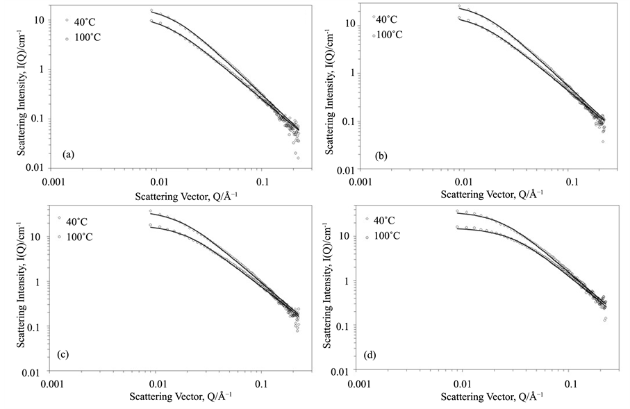
Figure A3. SANS profile for PMA3 in D-squalane (a) 0.0083 g∙cm−3, (b) 0.0148 g∙cm−3, (c) 0.0296 g∙cm−3, (d) 0.0706 g∙cm−3. Black lines through data points show model fits to data.