Journal of Signal and Information Processing
Vol.4 No.3(2013), Article ID:35610,15 pages DOI:10.4236/jsip.2013.43034
Spatial Image Watermarking by Error-Correction Coding in Gray Codes
![]()
Faculty of Science and Engineering, Toyo University, Kawagoe, Japan.
Email: kimoto@toyo.jp
Copyright © 2013 Tadahiko Kimoto. This is an open access article distributed under the Creative Commons Attribution License, which permits unrestricted use, distribution, and reproduction in any medium, provided the original work is properly cited.
Received May 8th, 2013; revised June 8th, 2013; accepted July 8th, 2013
Keywords: Gray Code; Error-Correcting Code; Digital Watermark; Spatial Domain; JPEG DCT-Based Compression
ABSTRACT
In this paper, error-correction coding (ECC) in Gray codes is considered and its performance in the protecting of spatial image watermarks against lossy data compression is demonstrated. For this purpose, the differences between bit patterns of two Gray codewords are analyzed in detail. On the basis of the properties, a method for encoding watermark bits in the Gray codewords that represent signal levels by a single-error-correcting (SEC) code is developed, which is referred to as the Gray-ECC method in this paper. The two codewords of the SEC code corresponding to respective watermark bits are determined so as to minimize the expected amount of distortion caused by the watermark embedding. The stochastic analyses show that an error-correcting capacity of the Gray-ECC method is superior to that of the ECC in natural binary codes for changes in signal codewords. Experiments of the Gray-ECC method were conducted on 8-bit monochrome images to evaluate both the features of watermarked images and the performance of robustness for image distortion resulting from the JPEG DCT-baseline coding scheme. The results demonstrate that, compared with a conventional averaging-based method, the Gray-ECC method yields watermarked images with less amount of signal distortion and also makes the watermark comparably robust for lossy data compression.
1. Introduction
Digital watermarking is a technique for uniting digital signals and additional data, which are commonly called watermarks, so as to make changes in the signals imperceptible [1]. As for image signals, a watermark is embedded into a source image in a manner such that the resulting degradation of image quality is hardly noticeable. The watermark is to be recovered afterward for verifying the ownership of the image, for instance. From the viewpoint of signal domains to directly modify for expressing watermarks, the watermarking techniques are mainly divided into two categories: spatial-domain-based techniques and transform-domain-based ones.
In transform-domain-based image watermarking, pixel values of a source image, which are expressed in quantized signal levels, are first transformed into frequencies using a signal transformation such as the discrete cosine transform (DCT). These frequencies are, then, modified so as to include a watermark. Lastly, a watermarked image is produced from the modified frequencies by the inverse transformation and re-quantization. The changes in frequencies made by the watermark are inversely transformed to the changes in pixel values and thereby, they are dispersed over the watermarked image in such a way that the image distortion can be less conspicuous. Quantizing errors, however, generally result from the re-quantization of the inverse transforms. These errors disturb the transform domain as a result. Hence, the watermark essentially needs to be embedded with redundancies in the transform domain. These redundancies can also lead to some extent of robustness of the watermarks against signal changes in the spatial domain.
In spatial-domain-based image watermarking, pixel values are directly modified so as to include a watermark. A well-known conventional method for this processing is to replace some bits of pixel values, which are assumed to be expressed in binary notation, with watermark bits. Accurate watermarks can thus be embedded without any such redundancies as that essential to the transform-domain-based watermarking schemes. Such changes in pixel values, however, directly distort the source image. In addition, the watermarked image generally has weak robustness to subsequent signal distortions because even a small change in a pixel value is likely to cause a significant change in the binary representation [2]. However, spatial-domain watermarks are nevertheless used in a number of applications such as steganography and fragile watermarking for content authentication.
As regards today’s digital systems, data are usually compressed for transmission, storage, etc. When a watermarked image is transmitted through an image communication system, the image is usually compressed by, for example, the JPEG coding scheme before transmission. Hence, when the image is recovered at the receiver, it is distorted due to the lossy data compression. Because such lossy data compression is a kind of usual processing in communication systems, if watermarking is carried out before transmission, the watermark must be robust against at least the distortion caused by a data compression method being in use.
Wang et al. proposed the pixel surrounding (PS) method as a spatial-domain-based image watermarking method, and reported that the watermarks embedded by the method can survive JPEG lossy compression [3]. The PS method reduces effects of signal distortions on the embedded watermark by averaging pixel values, which is a kind of low pass filtering. On the other hand, error correcting techniques in channel coding such as the BoseChaudhuri-Hockquenghem (BCH) codes [4] can be used to improve robustness of spatial-domain watermarks [5]. A number of the related coding methods were studied in the late 1990’s [2]. Most of such error-correction coding (ECC) methods have been applied to transform-domain watermarks [6].
With regard to signal bits, a quantized signal level is generally represented by a natural binary code, which is one of equal-length codes. Another equal-length code is the Gray code (also called the reflected binary code). This code has the property that any two adjacent codewords differ in only one bit position. Thus, small changes in a signal level are unlikely to affect all the bits of the codeword [7]. Accordingly, if the number of the changed bits is limited, they can be corrected by using error-correcting codes. In this paper, we consider watermarking by using both the Gray code to express the spatial domain and an error-correcting code to achieve robustness to signal changes. The objective of robustness here is to survive ordinary data compression such as the JPEG lossy coding.
The rest of this paper is organized as follows. Section 2 describes the codeword properties of Gray code. In the section, first, a single bit position where two adjacent codewords differ is given as a function of a signal level. Then, for each difference signal-level, the distribution of bit positions where two codewords just apart by the level from each other differ is demonstrated and compared with that in the case of the natural binary code. After formalizing the watermarking of signal codewords, Section 3 presents a scheme of error-correction coding in the Gray code representation. Based on the properties of the Gray code described in the preceding section, signal codewords involving single-error-correcting codewords are defined. The performance of error correction in the change of signal levels is verified by stochastic analyses. In Section 4, results of some experiments conducted on test images are presented to demonstrate performance of the proposed method, referred to as the Gray-ECC method, by comparison with the PS method. To begin with, the procedures for implementing the Gray-ECC method in image watermarking are defined. In addition, with regard to the PS method being compared, the implementing procedures are explained on referring to [3], and its properties depending on the parameter values are discussed to make a reasonable comparison with the ECC method. Then, both the image quality and the capability of robustness to JPEG lossy compression are evaluated from the experimental results. Section 5 concludes the paper.
2. Properties of Gray Code
2.1. Difference between Two Adjacent Codewords
First of all, we define the notation used in this paper. An m-bit Gray code is transformed from the natural binary code of the same length. Let Rm denote the decimal range of m-bit quantized levels , and let CR generally represent an m-bit binary code that consists of
  codewords corresponding to respective levels in Rm. The m-bit natural binary codeword
  for a level
 is just the binary representation of v; that is,
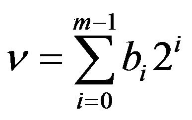 (1)
(1)
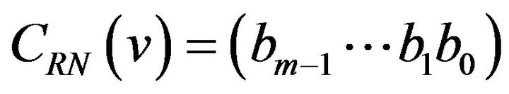
where bi is either 0 or 1 for . Let CRN denote the m-bit natural binary code and
  be the codeword in CRN associated with a level
 . The m-bit Gray codeword
  for a level v is calculated from the
  by the relation
 (2)
(2)
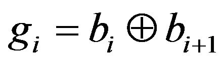
for . In Equation (2),
  denotes the exclusive OR operation, and bm that the equation needs is temporary here and supposed to be 0. Let CRG denote the m-bit Gray code and
  be the codeword in CRG associated with a level
 .
.
A bit position where two adjacent Gray codewords differ depends on the levels that the codewords represent. For a level v ( ), consider the codewords
 and
and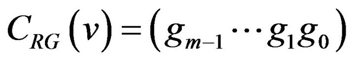 , and the respective succeeding codewords
  and
and
 . Then, the difference between
  and
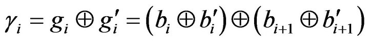
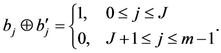
and  is expressed as the bit sequence
  that, by using Equation (2) with the associative and commutative laws of the exclusive OR operation, is given by the relations
 (3)
(3)
for . From another viewpoint, the least significant bits of any
  can be expressed as
 ; that is, a certain
  exists, and
  and
and for
for . Here, we define
  if v is even. Note that the corresponding bits in
  are
are . Then,
 4)
4)
Using this relation in Equation (3) yields
 (5)
(5)
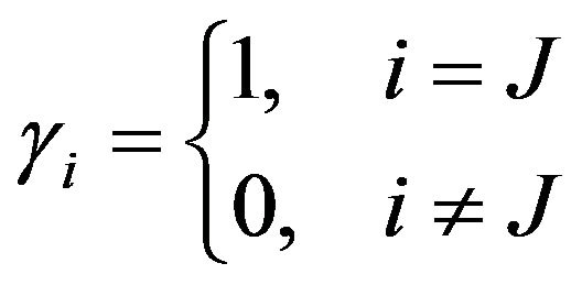
for . Thus,
  and
and  differ in only one bit
 , and J depends on the bit pattern of
  or equivalently, on the value of v. Consequently, the bit position J where
  and
and  differ is given by
 (6)
(6)
In addition, it is found that  if v is odd.
2.2. Difference between Two Codewords
The difference between  and
and where d (≥1) is a difference signal-level, is given by the result of accumulating bit changes from
  through
 . Hence, these two codewords differ in those bit positions where the bit inversion occurs once or odd times during the accumulation. For d ≥ 2, thus, one or more bits differ between the codewords, and the locations of difference bits are determined from the starting level v. Consequently, the distribution of difference bits in the entire m-bit codeword for all v’s that satisfy
  is derived using Equation (6).
Let m = 8 as a practical example. For d = 1, 128 even values of 255 v’s yield the difference bit g0’s between
 and
and . Out of the 127 possible codeword pairs of odd v, 64 pairs have the difference bit at g1, 32 pairs at g2, 16 pairs at g3, 8 pairs at g4, 4 pairs at g5, 2 pairs at g6, and one pair at g7. For d = 2, if v is even, then v + 1 is odd, and vice versa. As a result, any codeword pair has a difference bit g0 and another one; out of 254 possible codeword pairs, 128 pairs have the different g1, 64 pairs g2, 32 pairs g3, 16 pairs g4, 8 pairs g5, 4 pairs g6, and 2 pairs g7. For d = 3, in the case where v is even, in any one of 127 possible codeword pairs, the g0’s are same because v + 2 is also even, and the bits are different in one of the other seven bit-positions. For the other 126 pairs where v is odd, two codewords differ in three bit-positions composed of g0, g1 and one of the other six positions. Figure 1 illustrates the distributions of the difference bits in
  for each value of d from 1 to 8, for instance.
2.3. Comparison with Natural Binary Code
As for m-bit natural binary representations, the difference between two codewords is analyzed as below. The number, μ, of bit positions where two adjacent codewords differ ranges from 1 to m. For each μ, there are  possible codeword pairs, and any of the pairs differs in the bit positions from 0 through
 . For a difference signal-level d = 2, the number, also denoted by μ, of bit positions where two codewords
  and
and 
differ ranges from 1 to m − 1. There are  possible codeword pairs for each μ, and any of the pairs differs in the bit positions from 1 through μ while the b0’s are always the same. For a difference signal-level d = 3, the number of bit positions where two codewords
  and
and  differ ranges from 2 to m. The difference between the codewords gets more complicated than that for the above d = 2 or d = 1, while the b0’s are always different.
As the above examples demonstrate, for a given difference signal-level d, with regard to the pairs of codewords whose levels are apart by d from each other, the number of bit positions where two Gray codewords differ lies in a narrower range than that of bit positions where two natural binary codewords differ.
3. Error-Correcting in Gray Code
3.1. Formalization of Watermarking Codewords
The process of watermarking signals in code representations can be expressed in a generalized form as below.
1) Embedding process In addition to the notation used in the preceding section, we define the inverse mapping from CR to Rm, that
Figure 1. Distributions of difference bits between two 8-bit Gray codewords apart by a difference signal-level d from each other, for : Ndiff denotes the number of difference bits occurring in a codeword; the numbers written in the right side denote the total numbers of codeword pairs to which the bit distributions apply; the number written at each bit position in parentheses denotes the number of codeword pairs which differ at the position; the asterisks indicate those bit positions only one of which differs at the same time.
is,  for
for  by
by
 (7)
(7)
where a unique v is determined for each c since the code CR is a one-to-one mapping. As for a watermarking algorithm to be considered, let us regard both of the embedding of watermarks and the extracting of watermarks as kinds of point operations where the processing for any signal in a signal sequence depends only on the value of that signal. Also, for simplicity, we assume that one watermark bit is embedded in one chosen signal.
Suppose that a source signal sequence, X, and a watermark-bit sequence, W, are given. In the embedding process, first, the value vx of a given signal x in X is mapped to the codeword cx in CR; that is,
 . (8)
. (8)
Next, for a given watermark bit , a procedure, named EMBED, performs embedding w into cx; this is expressed in the form of a point operation such that
 (9)
(9)
where cy is the resulting codeword and . The signal value, vy, that cy represents is given by
 , (10)
and the source signal x is replaced with the signal of the level vy. Let Y denote the entire sequence of the replaced signals. Thus, the signal sequence X is changed to Y with the watermark W embedded there. The difference of the signal values vx and vy, which is generally referred to as an embedding distortion, degrades the signal quality of Y from X.
2) Extracting process Assume that, undergoing some signal processing such as data compression, the above sequence Y changes to another one, Z, of different signal values. In the watermark recovering process, a procedure for extracting watermark bits from codewords in CR is defined as the following inverse process of Equation (9): Referring to the procedure as EXTRACT, we can write it in the form of a point operation; that is, using the notation of Equation (9),
 . (11)
To extract the watermark from Z using this procedure, first, the value, vz, of each signal in Z is mapped to the codeword, cz, in CR; that is, similarly to cx of Equation (8),
 . (12)
Then, the procedure performs on cz as
 (13)
(13)
where w' is the resulting bit.
Robust watermarking requires w' to be equal to w in spite of the change in signal level from vy to vz. Howeverif , then obviously,
  because of the one-to-one mapping of the code. As a result, the change in codeword is likely to lessen the reliability of a watermark extracted from the resultant codeword.
It is clear from the above relations that the change in codewords affects directly the extraction of watermark bits. This also implies that for the purpose of recovering watermarks, it is sufficient to recover at least those bits of a codeword which affect the embedded watermark.
3.2. Single-Error-Correcting in Gray Code
When a signal changes by one level, one bit of the corresponding Gray codeword changes. Accordingly, the changed bit can be corrected by means of a single-errorcorrecting (SEC) code. Then, we employ single-errorcorrection coding in watermarking to make embedded watermarks completely robust against a change by one level in any signal.
1) Encoding procedure The processing of encoding watermark bits with a SEC code can be involved in the embedding operation EMBED of Equation (9). Let CE denote an error-correcting code to be used, which is assumed to be a linear block code in this paper, and nE be the code length of CE. For a signal level vx and a watermark bit w, given the corresponding codeword ,
, 
can be defined by the following two steps. Note that we still use a general notation of CR as the code that represents signal levels.
(EN.1) Generate a codeword, cw, in CE corresponding to the bit value of w.
(EN.2) Replace nE consecutive bits of cx from a specified bit position k (≥ 0) with all the bits of cw. Here, the bit position 0 designates the least significant bit (LSB). The resulting codeword is equivalent to cy of Equation (9). Let us define a REPLACE operator to implement the operation of this step in the form
 . (14)
In the above procedure, the codeword cx is changed depending on both cw and k. The change in codeword immediately affects the signal level and the resultant level vy is determined. To reduce the embedding distortion,  , a code CE of short codewords is desirable. A binary linear SEC code of the minimum code length is a (3, 1, 3) code consisting of two 3-bit codewords that are apart by the Hamming distance of 3 from each other and that correspond to respective values of an information bit 0 and 1. A typical (3, 1, 3) code is the so-called (3, 1) repetition code or also known as the general Hamming (3, 1) code [4]. Regarding each watermark bit as the information bit per codeword, we concentrate on a (3, 1, 3) code from now on.
2) Determining signal codewords Given a source signal and a watermark bit, to reduce the embedding distortion, from those codewords which include the error-correcting codeword corresponding to the watermark bit in the same bit-position, the one that results in the smallest embedding distortion must be chosen as the encoded codeword of the signal. The problem of choosing such codewords can be simplified in the way below.
Suppose that a (3, 1, 3) code  where the two codeword cE0 and cE1 correspond to respective watermark bits of 0 and 1 is given. Given a code CR for representing signal levels, for each value of watermark bit, putting the corresponding error-correcting codeword into all the codewords of CR by means of the REPLACE operator with a specified value of k, we obtain a subsetcode of CR, expressed in the form
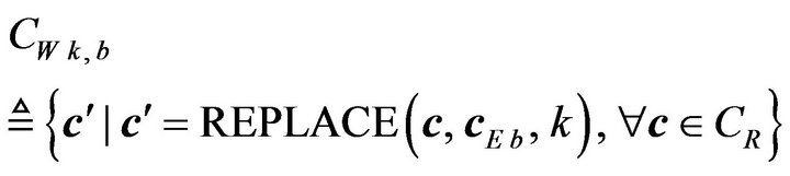 (15)
(15)
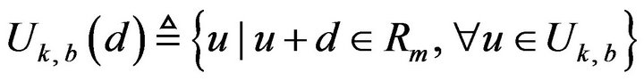
for b = 0 and 1 respectively. From each subset-code, a set of all signal levels that the codewords of the subset-code represent is obtained such that
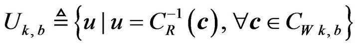 (16)
(16)
It follows that Uk,0 and Uk,1 are subsets of Rm. Thus, these subsets consist of signal values that each have had a watermark bit embedded by the error-correcting code.
For a given signal level  and a watermark bit
 , we choose such a level, vy, as closest to vx
from Uk, w. That is, vy is determined so that
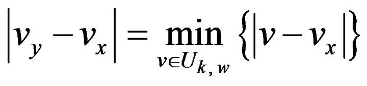 . (17)
It can be proved that in the case that the Gray code CRG is used as CR, the unique vy exists closest to each vx in either Uk,w. Let us denote the choosing operation of Equation (17) by the operator ENCODE in the form
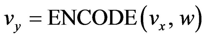 . (18)
This operator involves Uk, 0 and Uk, 1 that both have been made from CR and CE by Equations (15) and (16). The signals of a sequence X are thus encoded one by one to the single-error-correctable values, which compose the watermarked sequence Y.
3) Determining SEC codewords Since CE affects Uk, 0 and Uk, 1 through Equations (15) and (16), embedding distortions also depend on the codewords comprised in CE. On the assumptions that each level in Rm is equally likely to occur for any signal and also that a watermark bit is a random variable, for a given code  and a bit-position parameter k, the amount of embedding distortion can be estimated by calculating the expected value of the mean squared error (MSE) between the source signal levels and the encoded signal levels, defined by
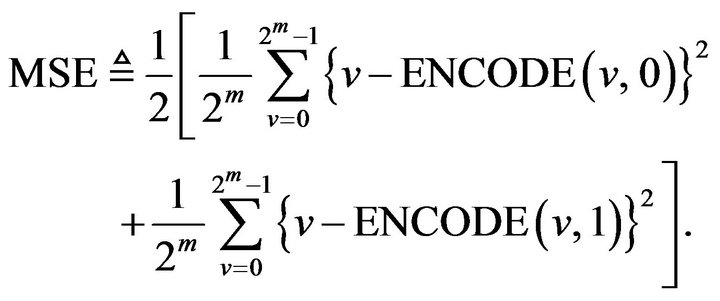 (19)
(19)
In fact, if CR has a periodic structure in codeword bits, the above ranges of summation can be reduced.
There exist the following four kinds of pair of 3-bit codewords that are apart from each other by Hamming distance of 3: (i) {(000), (111)}, (ii) {(001), (110)}, (iii) {(011), (100)}, and (iv) {(010), (101)}. Under the condition of using the Gray code CRG as CR, the expected MSE values of Equation (19) were calculated not only for each of the four codeword pairs but also for each bit position k of 0 and 1, respectively. The results are listed in Table 1, together with the peak-signal-to-noise ratio (PSNR) values in decibels (dB) defined by
 . (20)
On the above assumptions for stochastic analysis, the codes (i) and (iii) have exactly the same MSE values, and so do the codes (ii) and (iv) for both the bit positions. As shown in Table 1, the codes (i) and (iii) yield less distortion than the codes (ii) and (iv). On the other hand, as shown later, all the four codeword pairs have almost the same performance in error correction. Consequently, the codeword pair (iv) has been selected as CE for the Gray code; denoted by CEG, that is, . We refer to the encoding by the ENCODE operator with CEG and the position parameter k = 0 as ECCG0 and that with CEG and k = 1 as ECCG1. The encoding with the bit posi-

Table 1. Expected MSEs for (3, 1, 3) SEC codes embedded in Gray codes. (a) Bit position k = 0; (b) Bit position k = 1.
tion of k > 1 is no longer practical for 8-bit signals due to large embedding distortions.
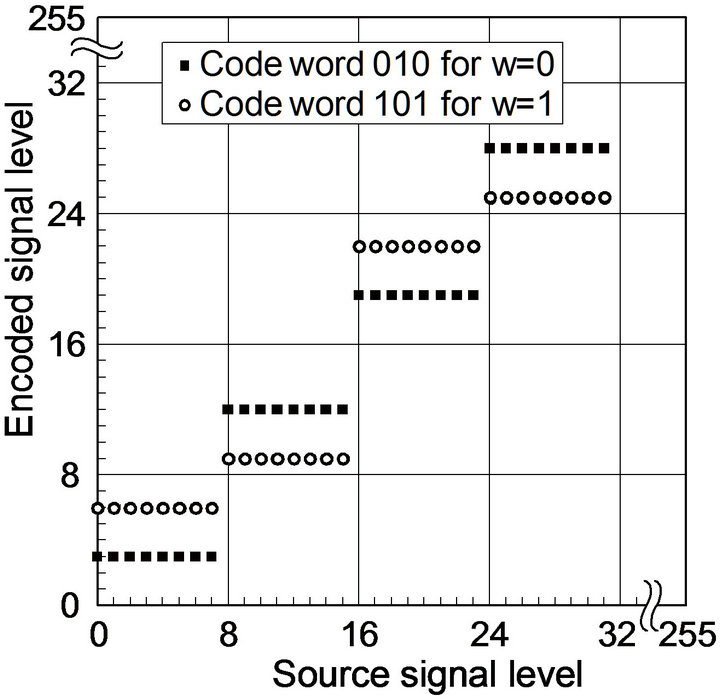
Figure 2 shows the relationship between source signal levels vx and encoded signal levels vy of Equation (18) in ECCG0 and ECCG1. The relationship in the interval of 16 source levels and that in the interval of 32 source levels repeat periodically over the 8-bit dynamic range for ECCG0 and ECCG1, respectively. In the period of ECCG1, the stepwise changes differ for the two codewords. With regard to embedding distortions, the magnitude of difference in signal levels caused by ECCG0 is less than or equal to 6, and that caused by ECCG1, less than or equal to 12.
4) Decoding procedure Given a signal sequence Z that has come from Y described in Section 3.2 (2), the process for decoding signal values to extract watermark bits is described as follows. Assume that both the error-correcting code
 and the bit-position parameter k that have been used for Y are known to the decoder. Let vz be the value of a signal z in Z, and let cz denote
 .
.
(DE.1) Obtain a codeword, e, from cz by separating nE
 (a)
(a)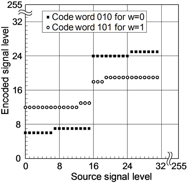 (b)
(b)
Figure 2. Source level-encoded level relationship of ECC methods. (a) ECCG0; (b) ECCG1.
consecutive bits starting at the bit position k. We define the operator SEPARATE that performs this bit-operation as
 (21)
(21)
where actually  for the (3, 1, 3) code CE.
(DE.2) The codeword e, which might have been distorted, is supposed to be decoded by using CE. To implement the decoding, assuming all distorted codewords are equally likely, we use a maximum-likelihood decoding method [4]. By the method, e is mapped to one of the two codewords cE0 and cE1 such that is closer to e than the other in terms of the Hamming distance. Let e' be the resulting codeword.
(DE.3) The bit value, w', corresponding to e' in CE is immediately obtained as the watermark bit extracted from vz.
We express the procedure that performs the above three steps for a given vz by the operator DECODE of the form
 (22)
(22)
which is implicitly associated with CE and k.
3.3. Stochastic Analysis of Error-Correcting Performance
Error-correcting performance of ECCG0 and ECCG1 are revealed by stochastic analysis below.
1) Error-correcting capabilities for a single levelchange For each encoded signal level  where k is given and
 , given a difference signal-level d satisfying
 , whether the result of decoding u + d, that is,
  agrees with b or not is determined. The agreement between the two bits b and b' depends on the difference between the two error-correcting codewords, cEb of
  and a' of
  that is obtained by
 (23)
(23)
If the Hamming distance between cEb and a' is either 0 or 1, then a' is mapped to cEb in the decoding procedure and thus, b' agrees with b. Otherwise, a' is mapped to the other error-correcting codeword , where
  denotes the 1's complement of b, and consequently, b' is regarded as
 .
.
Because the difference bits between two signal codewords  and
and  depend on the u in
 , we define a ratio of the correctly decoding of signals for the entire
  as follows. First, the whole of those values of
  which are allowed to increase by d within Rm is described by a set,
  , such that
 . (24)
Then, out of the values in , a set,
  of those values which, after increasing by d, still contain correctly decodable error-correcting codewords is expressed in the form such that
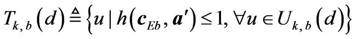 (25)
(25)
where a' is the same as that of Equation (23) and  denotes the Hamming distance between two codewords x and y. Supposing that signal values in
are equally probable, we estimate the probability of the correctly decoding of  for a variable d, denoted by
 , by the ratio
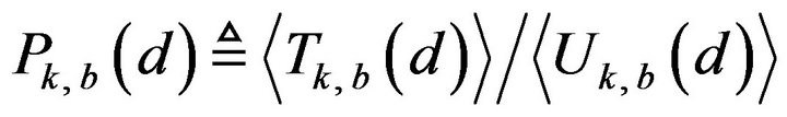 , (26)
where  denotes the number of elements in a set S, for b = 0 and 1, and k = 0 and 1 according to Section 3.2 (3).
On the additional assumption that watermark bits are random variables, an estimate of the correctly decoding probability of ECCGk, for k = 0 and 1, can be defined as follows. For the definition,  and
and  of the same d are put together by taking the average of the two values on the assumption that a signal change by d levels and that by −d levels are equally likely to happen to any level in
 . In fact, because of the symmetrical structure of Gray code, it holds that
 and
and  for any possible d and each b. Then, the overall probability of correctly decoding by ECCGk for a variable d, denoted by
 , is defined by
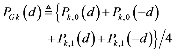 , (27)
where d > 0 .
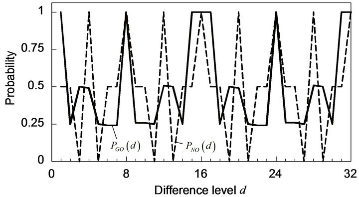
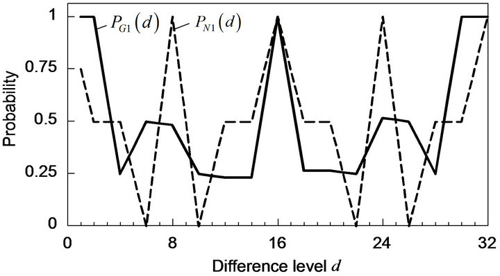
As regards ECCG0, Figure 3(a) shows the variation of
 with d, where let
 , for instance. In this case,
  , for b = 0 and 1, and for any possible d, and they have one of three values 0, about 0.5 and 1 if d is so small that
 , the denominator of Equation (26), is composed of a lot of elements. As shown in Figure 3(a),
  for any d, and
  has one of three values about 0.25, about 0.5, and 1. Particularly for
 ,
, .
.
For comparison, we define a (3, 1, 3) code, denoted by CEN, to use for the natural binary code CRN. Two codewords in CEN have been determined from MSE values similarly to those in CEG; that is,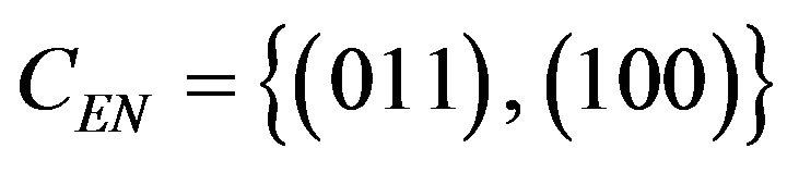 .
.
We refer to the encoding by the ENCODE operator with CEN as the natural ECC method, and let ECCNk denote the natural ECC method with the position parameter k, where practically  or 1. Note that no operation is actually needed for the transformation between m-bit binary signal values and m-bit codewords in CRN. Also, the expected probability of correctly decoding by ECCNk for a difference signal-level d, denoted by
 , is defined similarly to
 , for
, for  and 1 respectively. The variation of
  with d is added in Figure 3(a) by the broken line. For any possible d, each of
  and
and  has either 0 or 1, for
  and 1, and consequently,
  has one of three values 0, 0.5 and 1. Particularly for
 ,
, .
.
2) Error-correcting capabilities for multiple levelchanges The decoding properties are estimated under the condition that all the changes up to d levels occur in the en-
 (a)
(a) (b)
(b)
Figure 3. Performance of Gray-ECC in comparison with natural ECC for codeword position of 0 (k = 0). (a) Correctly decoding probabilities; (b) Accumulative probabilities.
coded signals. For the estimation, supposing that all the difference signal-levels in the range from 1 to d are equally likely, we define the accumulative probability of correctly decoding by ECCGk, denoted by  in the form of a function of d, by averaging from
  through d; that is,
 , (28)
for  and 1 respectively. Similarly to
 , the accumulative probability of correctly decoding by ECCNk, denoted by
 , is defined for each
  and 1.
The variation of  with d is shown in Figure 3(b), where let
 , with the variation of
  depicted for comparison by the broken line.
  is found to be greater than 0.5 for
 . Hence, ECCG0 is expected to achieve the error correction in this range of d. As the figure shows, with increasing d,
  gets close to 0.5. In contrast,
  for any d. This result indicates that ECCN0 has no capacity of correcting errors for those signals which have undergone change by various levels.
Effects of selected codewords in CEG on the errorcorrecting performance have been also evaluated. For this purpose, by replacing the codeword pair in CEG with each one of the three other codeword pairs (i), (ii) and (iii) previously mentioned in Section 3.2 (3), both the corresponding  and
and  were calculated. In comparison among the four codeword-pairs, the variations of these probabilities with d have been found to be almost the same. Consequently, the four codeword-pairs have no difference in error-correcting performance.
3) Bit position of error-correcting codewords For the bit position , the performance of ECCG1 has been evaluated. The variation of with d is shown in
Figure 4(a), compared with that of . In ECCG1,
  for
for  and 1, and for any possible d; they have one of five values 0, about 1/4, about 1/2, about 3/4 and 1. As Figure 4(a) illustrates, accordingly,
 has one of five values about 1/4, about 3/8about 1/2, about 5/8 and 1. Particularly for
  as well as
 ,
, . In addition, the variations of
  and
and  with d are both depicted in Figure 4(b). As this figure shows,
  becomes greater than 0.5 for
 . This range of d is much wider than that in ECCG0. Figure 4 also indicates that the fact
 results in that
  for
for .
.
 (a)
(a)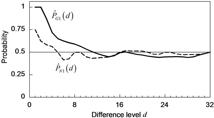 (b)
(b)
Figure 4. Performance of Gray-ECC in comparison with natural ECC for codeword position of 1 (k = 1). (a) Correctly decoding probabilities; (b) Accumulative probabilities.
Hence, ECCN1 is barely expected to achieve the error correction in this range of d.
From the above stochastic analyses, the advantages of the Gray code over the natural binary code in the ECC method are summarized as follows:
a) For any d,  while
while  for some of d’s.
b) For a given k,  for some of d’sin particular for
 .
.
These advantages result from the limited distribution of bit positions where two codewords differ as described in Section 2.2. Because of the advantages, ECCGk achieves the capability of correcting “errors”, namely signallevel changes particularly if the changes are limited in a small range.
4. Experiments
4.1. Watermarking Procedures
The procedures for implementing the ECC method, which means both the Gray-ECC and the natural ECC by generalization, is introduced in this section. Source images are assumed to be monochrome images or signals of one channel of color images, and a signal level of each pixel is represented by an m-bit code in natural binary notation. Using a general notation, for an image f, let  denote a pixel, or equivalently a pixel value at the coordinates
  on the image plane. A watermark is a sequence of bits, and the bits are supposed to be embedded into a source image one by one in order.
1) Embedding procedure Given a source image, fX, of the size NX by NY pixels and a watermark-bit sequence where NW is the number of watermark bits
 and
and for
for the embedding procedure performs according to the following steps:
(WE.1) Choose NW points ,
,
 , out of the coordinates of fX in a manner such that all the NW points are situated separately on the image plane. Let the sequence of the ordered points be represented by K; that is,
 .
.
(WE.2) According to K, obtain a pixel sequence, X, from fX; that is,  where
where
 for
for .
.
(WE.3) For each pixel xi in X,  , encode the pixel value with a given watermark bit wi using the operator ENCODE of Equation (18), so that
 . (29)
Then, replace the value of xi with vi. Expressing the resultant pixel by yi, we thus obtain the sequence
 .
.
(WE.4) Substitute yi in Y for the pixel at  in the image fX for
 . Thereby the watermarked image, fY, is achieved.
The sequence K is supposed to be associated with each fY, and it must be protected from unauthorized use. We here refer to the ratio of NW to the number of pixels in fX as an embedding pixel ratio ; that is,
 . (30)
2) Extracting procedure Given an image, fZ, that is assumed to be derived from the above fY, the procedure for extracting watermarks from fZ is as follows:
(WD.1) Using the same K as that has been used in the embedding procedure for fX, obtain a pixel sequence, Z, from fZ; that is,  where
where  for
for ,
,  .
.
(WD.2) For each pixel zi of Z,  , decode a bit, w'i, from the pixel value using the operator DECODE of Equation (22). We thereby obtain the bit sequence
 .
.
4.2. Pixel Surrounding Method
The performance of the proposed ECC method has been compared with that of the conventional pixel surrounding (PS) method [3]. The procedures of the PS method are outlined below. In addition, our analysis will reveal its essential properties in terms of embedding distortions and robustness.
1) Embedding procedure Given a source image fX and a sequence of NW watermark bits, the embedding procedure is as follows:
(PE.1) As in the step (WE.1) of the ECC method, determine a sequence of NW points in fX. Let K denote the sequence, and the same notation as that in the ECC procedure is used here.
(PE.2) According to K, obtain a sequence, X, of NW pixels from fX.
(PE.3) Foreach xi in X, calculate the mean value, ai, of the eight pixels surrounding xi in the neighborhood of 3 by 3 pixels. Thus, a sequence 
is obtainedfor all .
.
(PE.4) For the ith watermark bit , replace the signal value of xi with
  such that
 (31)
(31)
for , where
  is a specified positive value of signal level. Letting x'i denote the resultant pixel, we thereby obtain a pixel sequence
 .
.
(PE.5) Substitute x'i in X' for the pixel at  in the image fX. Let
  be the resulting image, so that
 for
for .
.
2) Extracting procedure The procedure for extracting watermarks from a given image,  , that is supposed to come from the above
  is as follows:
(PD.1) Using K that has been determined in the step
(PE.1), obtain a pixel sequence, Z, from ; that is,
  where
where  for
for ,
, .
.
(PD.2) For each zi in Z, calculate the mean value, a''i, in the neighborhood of zi in the same way as in the step
(PE.3). Then, a sequence  is obtained.
(PD. 3) By comparing the signal value 
with a''i, a bit value, w''i, is determined in a manner such that
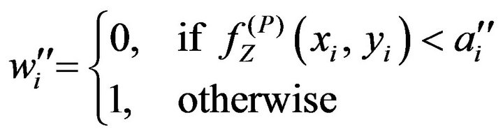 (32)
(32)
for . Thus, the bit sequence
 is obtained as a watermark extracted from
 .
.
3) Embedding distortions Embedding distortions caused by the PS method are signal changes at the embedding points. To estimate the amount of the distortion, we use the measurement of MSE between the two images fX and , expressing it by MSEPS. The general definition of MSE between two images f1 and f2 of the same size of NH by NV pixels is
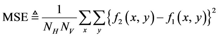 (33)
(33)
where the summation is taken over the entire image area. Replacing f1 and f2 in Equation (33) with the respective images of fX and  yields directly the form of MSEPS.
Based on the definition, the value of MSEPS for a given  is approximately proportional to the embedding ratio. Using MSEPS instead of MSE in Equation (20), we can also obtain the value of PSNR.
At each of the embedding points in , the pixel has a value different from the average of its neighborhood pixels by
  according to Equation (31). Then, the pixel value can be regarded as the sum of the spatial average and a noise signal that is randomly chosen between
  and
and  on the assumption that the watermark bits are random variables. Hence, the image
  gets closer to a result of spatial averaging with decreasing
 , and accordingly, it looks more blurring, particularly when the embedding pixel ratio is large and close to 1.
4) Robustness In the step (PE.3) of the above embedding procedure, the neighborhood averaging is carried out using source signal levels of fX and hence, the resulting average at each point is independent of the situations of any other points of K. In addition, the steps (PE.4) and (PE.5) are implemented by point operations. Accordingly, the steps from (PE.2) through (PE.5) can be accomplished by a parallel processing with the 3 by 3 operator applied to fX
at each point of K. The pixels of  are consequently generated from fX independently of each other.
On the other hand, in the extracting procedure, the step (PD.2) involves the calculation in the neighborhood in
 around each point of K. This spatial operation makes the mean value calculated at each point dependent on the situations of the other points of K as described below. Suppose that a point of K, say,
  , has its neighbors including another point of K, say,
 .
.
Also, suppose a mean value, a'j, calculated in the neighborhood around  in
in . Then, a'j is no longer equal to aj obtained in the step (PE.3) due to the difference between the level of
  and
and .
.
The difference between the mean values aj and a'j has a certain effect on the performance of watermark extraction. The condition for extracting correct watermark bits from  is given from Equation (32) as
 where
where . This interval of
  just depends on
 . If
. If  is larger than
 , either a watermark bit of 1 or that of 0 is unable to recoveraccording to whether
  is positive or negative. Henceall the watermark bits would be hard to recover even from the watermarked and still unchanged image without any limitation of the situations of embedding points. The condition sufficient for correctly recovering all the watermark bits is that every point of K is situated outside the 3 by 3-pixel neighborhoods of any other points of K. Note that satisfying this condition makes the embedding pixel ratio
  unable to exceed 1/9.
As for a processed and probably changed image let us express the pixel values and the mean values calculated in the step (PD.2) by the relations
 (34)
(34)
and
 (35)
(35)
respectively, for . Substituting these expressions in Equation (32), we find that if
 where
where , the watermark bit of either value is to be correctly extracted from
 . If
. If , the watermark bit of 1 is lost, and otherwisethe watermark bit of 0 is lost.
4.3. Experimental Methods
The experimental procedure that was carried out to evaluate the ECC method is described here. Some 8-bit monochrome images of 256 by 256 pixels, such as commonly used “Lena,” were used as source images in the experiment. The embedding of watermark bits was carried out for all the pixels of a source image so that the performance with the upper limit of the embedding pixel ratio, that is,  could be evaluated. Note that the watermarking is actually to be implemented with
  to hide where watermarks are embedded. As an instance of watermark, W, a sequence of 256 × 256 bits was generated using a pseudo-random number generator with a computer, and thus,
  where
where
 .
.
The procedure applied to each source image, fX, consists of the following steps:
(EX.1) Embed W into fX by the ECC method. Let fY denote the resulting image. Then, measure a PSNR value between fX and fY.
Here, ECCG0 and ECCG1 were used as the Gray-ECC method, and also, ECCN0 and ECCN1 were used for comparison. Furthermore, the PS method was implemented for fX with  and various values of
 . Thus the respective fYs were produced from each fX by these methods.
(EX.2) Compress fY using the JPEG DCT-baseline system, and decompress the resultant data to reconstruct an image, fZ. Then, measure a PSNR value between fY and fZ to estimate the amount of distortion caused by the JPEG lossy compression.
To obtain various amount of distortion, the JPEG coding performance was varied by multiplying the entire luminance-quantization matrix that is specified as the recommended one in [8] by a constant and thus, several fZs with the various distortions were produced for each fY.
(EX.3) Extract a watermark-bit sequence from fZ using the decoding procedure corresponding to each embedding method. Let the resulting bit-sequence be
 .
.
We define a watermark-bit correct ratio, RC, of fZ as the ratio of correct watermark bits among those extracted from fZ. Using the above W and W', it can be calculated by
 . (36)
RC of fY can be defined similarly from a watermark-bit sequence extracted from fY.
As described in the step (EX.1), all the methods are compared under the condition that the embedding pixel ratio . As for other values of
 , due to the point operation in these methods, generally, MSE values between fX and fY defined by Equation (33) vary almost in proportion to
  of fY for each fX.
4.4. Experimental Results and Discussion
1) Quality of watermarked images

Table 2(a) lists PSNR values of the watermarked images fY obtained by applying each of the ECC methods to four different source images fX: “Lena,” “Aerial,”
Table 2. Embedding distortions by ECC methods. (a) PSNR (dB); (b) WSNR (dB).
“Peppers”, and “Parrots”. Compared among these images, the PSNR values given by each method are almost the same; the PSNR values given by ECCG0 and those given by ECCG1 agree well with the respective values obtained by the stochastic analysis (previously shown in Table 1), and so do the PSNR values given by ECCN0 and ECCN1. On the average, PSNR values of the results of ECCG1 are about 5.5 dB smaller than those of the results of ECCG0 for any test image; PSNRs of the results of ECCGb are about 2 dB smaller than those of the results of ECCNb for  and 1. Note that RC of fY by any ECC method is equal to 1.
In addition, weighted signal-to-noise ratio (WSNR) values were calculated from the difference between fY and fX. In the calculation, the viewing distance of 13 inches and the image resolution of 200 pixels per inch were assumed. Table 2(b) lists the WSNR values of the results of each ECC method for the four test images. On the average in the ECC methods, each watermarked image has a WSNR value 3.7 dB larger than the PSNR value.
With regard to the PS method, Table 3(a) shows PSNR values and RCs of fY obtained by the experiment using the four test images with  and various values of
 ; Table 3(b) shows those values for
  and some values of
 ; Table 3(c) shows WSNR values for
  and some δs. The results for
  in Table 3(a) demonstrate that the PSNR values are substantially small and more than 10 dB smaller than those of ECCG0 even for
 . Increasing
  decreases the PSNR values whereas achieving large values of RC requires
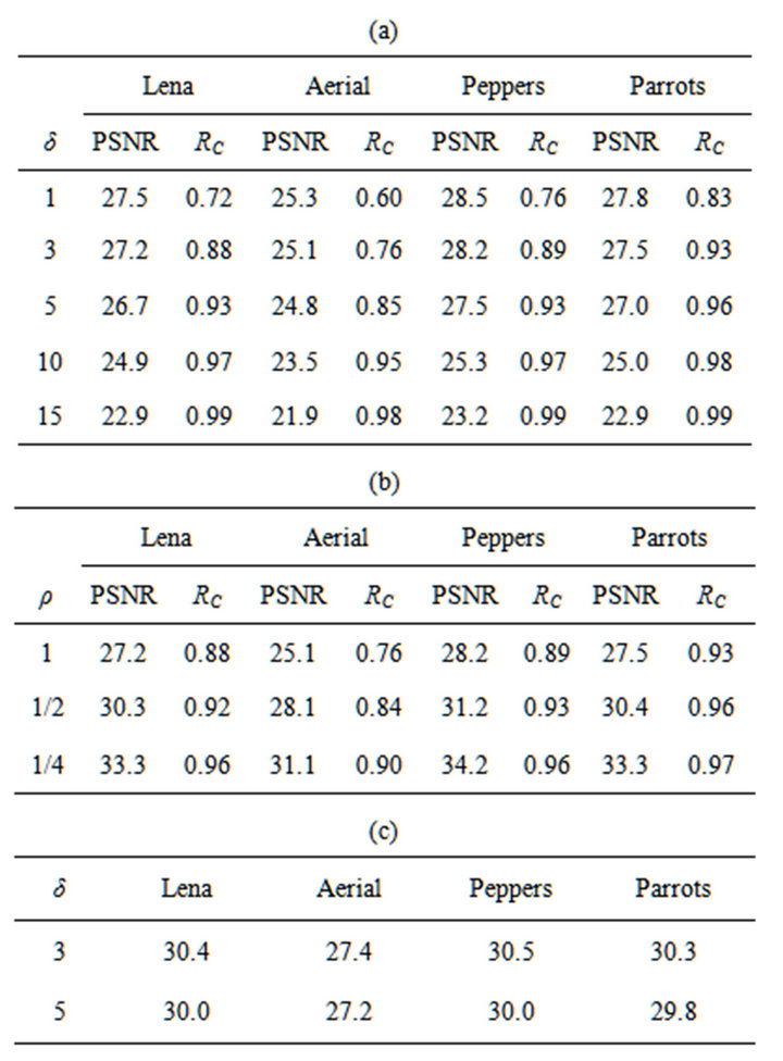
Table 3. Watermarking results of PS method. (a) PSNR (dB) and RC with ρ = 1; (b) PSNR (dB) and RC with δ = 3; (c) WSNR (dB) with ρ = 1.
large values of . It is also revealed from Table 3(b) that for any of the test images, although the PSNR value increases linearly with decreasing
  as expected, it is still small even for
 : The PS method with
  and
and  is comparable to ECCG1 in terms of PSNR. Also, from a comparison between Tables 3(a) and (c), we find that each watermarked image has a WSNR value, on the average, 2.7 dB larger than the PSNR value.
To evaluate image appearance, Figure 5 shows examples of the watermarked images. The ECCG0 hardly yields perceptible distortions on the resulting images as shown in Figure 5(b). As seen in Figure 5(c), on the contrary, the ECCG1 tends to generate visible artifacts similar to “false contours” [7] particularly in areas of smooth gray levels. As for the PS method, the image degradation is mainly due to the averaging operation, which is a kind of low-pass filtering: the watermarked images of small δs as shown in Figure 5(d) look considerably blurred; the images of large δs look grainy as well as blurred as seen in Figure 5(e).
2) Error-correcting capability The error-correcting capabilities of the ECC methods for signal changes were evaluated from the experimental
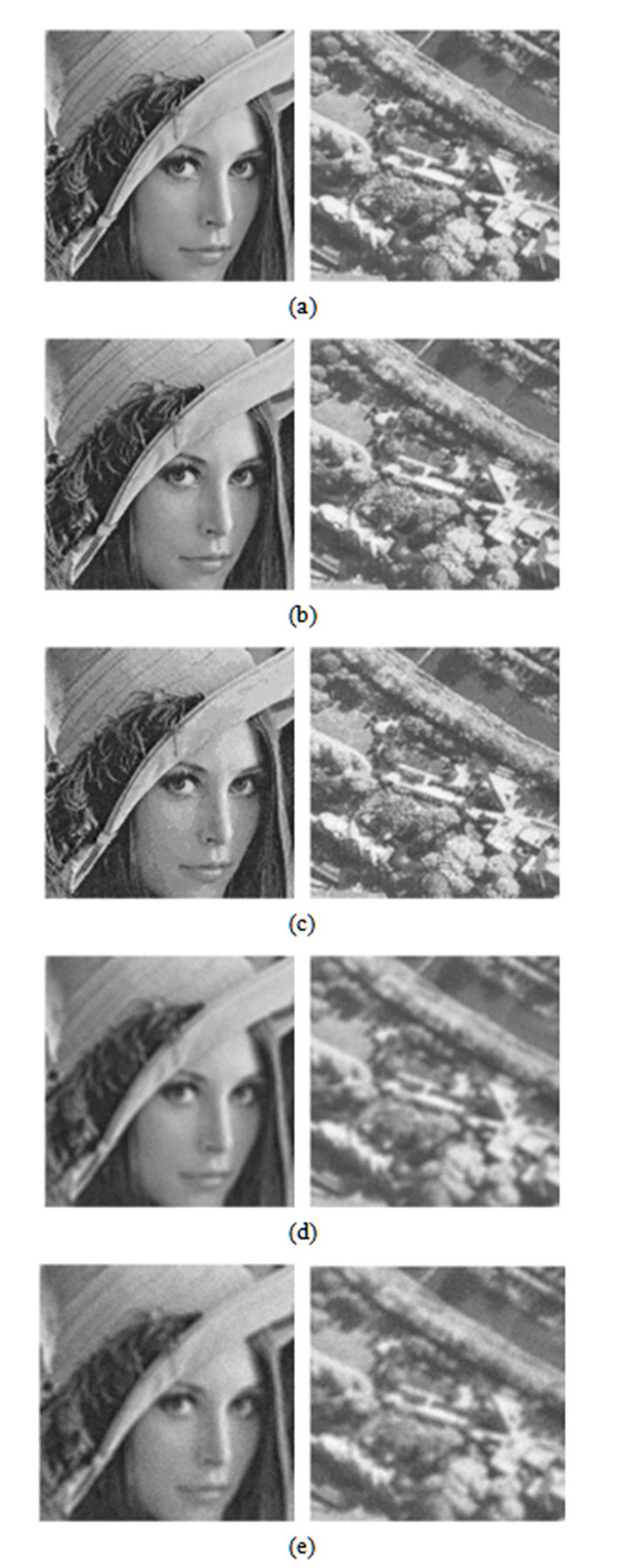
Figure 5. Examples of images “Lena” (left) and “Aerial” (right): (a) source images; results of watermarking (b) by ECCG0, (c) by ECCG1, (d) by PS method with ρ = 1 and δ = 3, and (e) by PS method with ρ = 1 and δ = 5. All the images show the 128 by 128-pixel section centered in their respective images.
results. As a measure of the capability, we define a error-correction success ratio, RS, of fZ for fY as the ratio of those pixels from which correct watermark bits are able to be extracted among those watermarked pixels of fZ whose signal levels differ from those of fY. To formulate RS for calculation, let Kerr be a set of locations of those watermarked pixels whose values differ between fY and fZ; that is,
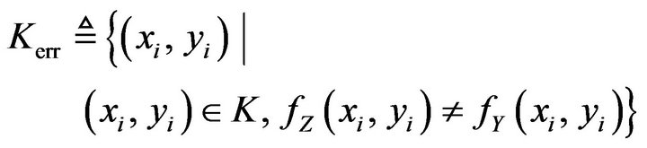 . (37)
Then, using the original watermark W and the extracted W', RS can be calculated by
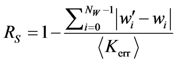 (38)
(38)
where  represents the number of elements of Kerr.
Before evaluating error-correcting performance, we examine the amount of signal distortion caused by JPEG compression. Figure 6 shows examples of occurrence frequencies of difference levels between a JPEG-compressed image and its source image for various degrees of data compression. As this figure demonstrates, the difference levels tend to concentrate into small ones and also, the range is limited to a few levels particularly in the distorted images of PSNR larger than 40 dB.
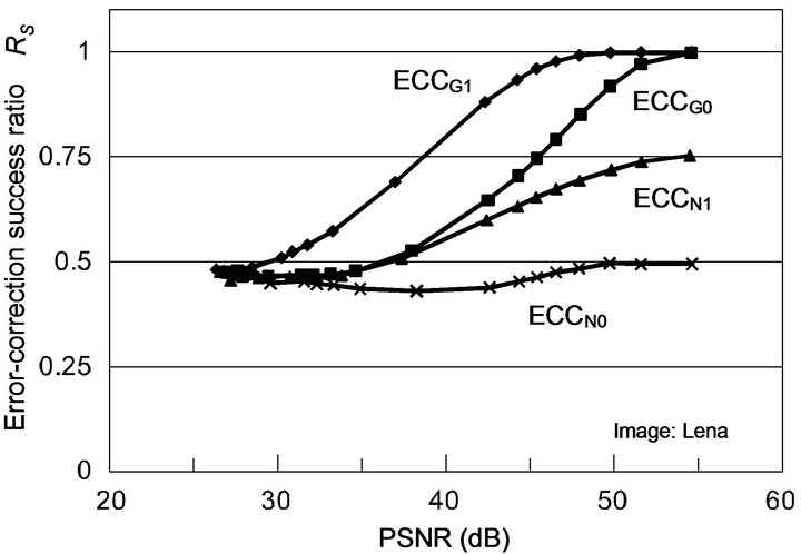
Figure 7 shows the experimental results for two test images, depicting variations of RS with PSNR values of JPEG-compressed images for each of the ECC methods. Both the images have almost the same result. These experimental results agree well with the stochastic analyses described in Section 3.3: As the PSNR value increases, the MSE value equivalently decreases, and accordingly, the difference levels concentrate in a narrow range as Figure 6 has shown. Hence, the accumulative probability of correct decoding can explain the variation of RS: RS values of ECCG0, ECCG1, ECCN0 and ECCN1 get close to
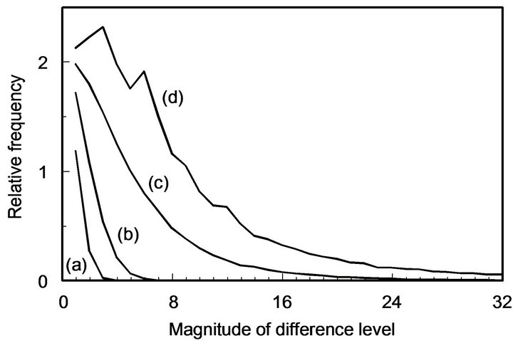
Figure 6. Examples of distribution of difference levels in JPEG compressed images: The source image to JPEG encoder is “Lena” watermarked by ECCG0; JPEG compressed images have respective PSNRs of (a) 48.0 dB, (b) 42.5 dB, (c) 31.4 dB, and (d) 27.0 dB; The relative frequency of difference level d is defined as the ratio of the number of pixels of difference level d to the number of unchanged pixels in each image.
 (a)
(a)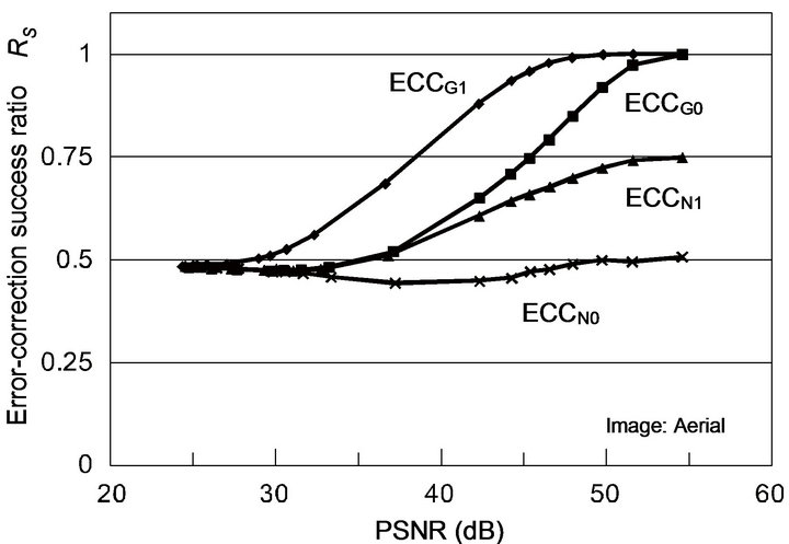 (b)
(b)
Figure 7. Variation of error-correction success ratio with amount of signal distortion caused by JPEG lossy compression for the test image (a) “Lena” and (b) “Aerial.”
the respective values of ,
,  ,
,  and
and , which have been shown in Figures 3(b)
and 4(b). In Figure 7, ECCG0 and ECCG1 have RS over 0.5 beyond about 35 dB and 30 dB, respectively, and achieve RS over 0.9 above about 50 dB and 45 dB, respectively. Thus, these two methods have the capability of error correction for JPEG distorted images. In contrast, ECCN0 is unable to afford the error correction for any distribution of difference levels; ECCN1 has RS values greater than 0.5 and as much as 0.75 beyond about 37 dB.
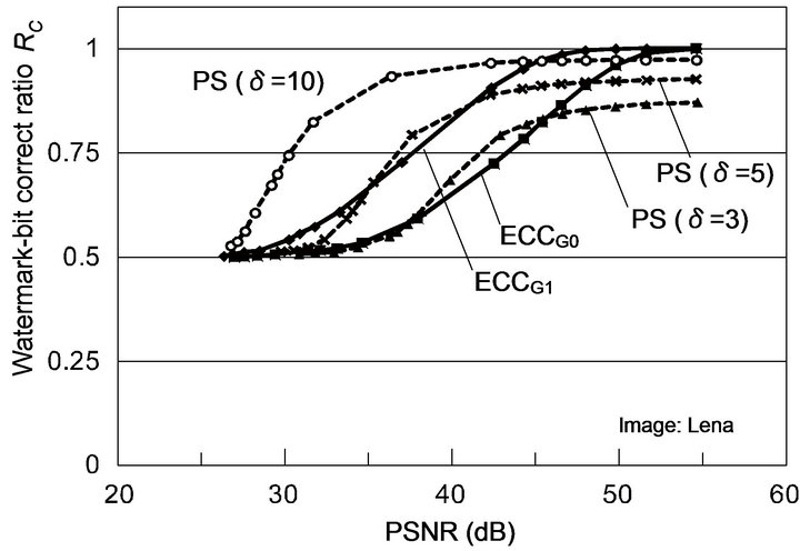
3) Robustness for JPEG lossy compression
Figure 8 shows the experimental results for two test images, depicting variations of RC with PSNR values of JPEG-compressed images for ECCG0 and ECCG1. As regards these ECC methods, both the images have almost the same result. These results indicate that correct watermark bits can be recovered from JPEG-distorted images of PSNR of over 30 dB by either Gray-ECC method.
Figure 8 includes the results of the PS method with  and
and , 5, and 10 for comparison. In accor-
 (a)
(a)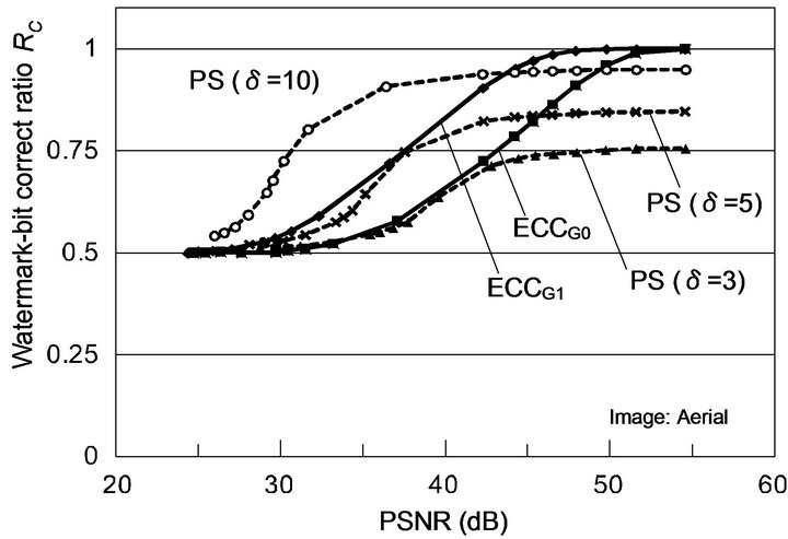 (b)
(b)
Figure 8. Variation of watermark-bit correct ratio with amount of signal distortion caused by JPEG lossy compression for the test image (a) “Lena” and (b) “Aerial.”
dance with Table 3, RC values for the image “Lena” are larger than those for the image “Aerial.” Figure 8(a) implies that the performance of ECCG0 is comparable to that of the PS method with  in the range of about 35 to 45 dB, and the performance of ECCG1, that of the PS method with
  in the range of about 35 to 40 dB. To obtain a better performance than that of ECCG1, the PS method needs to be implemented with a large
  value such as 10 at the expense of enormous embedding distortions.
5. Conclusions
In this paper, the error-correction coding in Gray codes (ECC-in-Gray) has been considered to enhance the errorcorrecting capabilities, and its performance has been evaluated using the Gray-ECC method where ECC-in-Gray is applied to the protection of image signals watermarked in the spatial domain. The stochastic analyses and the experimental results have shown that although level changes caused by error-correcting codewords are somewhat enlarged by the transformation from Gray to natural binary codes, ECC-in-Gray is suitable for distorted signals of such error-distribution as caused by lossy data compression.
The performance of the Gray-ECC method is summarized in comparison with that of the PS method as follows:
1) The Gray-ECC method has robustness against signal distortions caused by JPEG lossy compression comparable to that of the PS method.
2) The Gray-ECC method yields a considerably smaller amount of embedding distortion than the PS method in terms of PSNR.
3) The embedding distortion caused by the Gray-ECC method looks similar to the signal distortion by coarse quantization and tends to get noticeable particularly in smooth image areas. As for the PS method, the watermarked images primarily look blurred because of the use of neighborhood averaging, and increasing the capacity of robustness makes the image appearance grainier.
ECCG1 has stronger robustness than ECCG0, but it possibly yields more perceptible distortions in smooth image areas. From this point of view, effectively robust watermarks are expected to be achieved by switching between ECCG0 and ECCG1 for each image area depending on, for example, the degree of smoothness of the area. Such an adaptive system will be a subject in the further study.
REFERENCES
- B. M. Macq, “Special Issue on Identification and Protection of Multimedia Information,” Proceeding of the IEEE, Vol. 87, No. 7, 1999, pp. 1059-1276.
- I. J. Cox, M. L. Miller and J. A. Bloom, “Digital Watermarking,” Morgan Kaufmann Publishers, San Francisco, 2002.
- F. H. Wang, J. S. Pan and L. C. Jain, “Innovations in Digital Watermarking Techniques,” Chapter 4, SpringerVerlag, Berlin, 2009. doi:10.1007/978-3-642-03187-8
- G. Clark Jr., and J. Cain, “Error-Correction Coding for Digital Communications,” Plenum Press, New York, 1981. doi:10.1007/978-1-4899-2174-1
- J. R. Hernández, F. P. González and J. M. Rodriguez, “The Impact of Channel Coding on the Performance of Spatial Watermarking for Copyright Protection,” Proceedings of the 1998 IEEE International Conference on Acoustics, Speech, and Signal Processing, Seattle, May 1998, pp. 2973-2976.
- Y. Yi, M. H. Lee, J. H. Kim and G. Y. Hwang, “Robust Wavelet-Based Information Hiding through Low-Density Parity-Check (LDPC) Codes,” In: T. Kalker, I. J. Cox and Y. M. Ro, Eds., Digital Watermarking, Springer-Verlag, Berlin, 2004, pp. 117-128. doi:10.1007/978-3-540-24624-4_9
- R. C. Gonzalez and R. E. Woods, “Digital Image Processing,” Addison-Wesley, Boston, 1993.
- ISO CD 10918, “Digital Compression and Coding of Continuous-Tone Still Images,” ISO/IEC JTC1/SC2/ WG10, 1991.