Journal of Signal and Information Processing
Vol. 4 No. 1 (2013) , Article ID: 28281 , 9 pages DOI:10.4236/jsip.2013.41004
Denoising of an Image Using Discrete Stationary Wavelet Transform and Various Thresholding Techniques
![]()
College of Computer Engineering & Science, Salman bin Abdul Aziz University, Al-Kharj, Saudi Arabia.
Email: syedamjadali.lords@gmail.com
Received August 13th, 2012; revised September 14th, 2012; accepted September 29th, 2012
Keywords: Wavelet; Discrete Wavelet Transform; Wavelet Packet Transform; Stationary Wavelet Transform; Thresholding; Visu Shrink; SURE Shrink; Normal Shrink; Mean Square Error; Peak Signal-to-Noise Ratio
ABSTRACT
Image denoising has remained a fundamental problem in the field of image processing. With Wavelet transforms, various algorithms for denoising in wavelet domain were introduced. Wavelets gave a superior performance in image denoising due to its properties such as multi-resolution. The problem of estimating an image that is corrupted by Additive White Gaussian Noise has been of interest for practical and theoretical reasons. Non-linear methods especially those based on wavelets have become popular due to its advantages over linear methods. Here I applied non-linear thresholding techniques in wavelet domain such as hard and soft thresholding, wavelet shrinkages such as Visu-shrink (nonadaptive) and SURE, Bayes and Normal Shrink (adaptive), using Discrete Stationary Wavelet Transform (DSWT) for different wavelets, at different levels, to denoise an image and determine the best one out of them. Performance of denoising algorithm is measured using quantitative performance measures such as Signal-to-Noise Ratio (SNR) and Mean Square Error (MSE) for various thresholding techniques.
1. Introduction
In many applications, image denoising is used to produce good estimates of the original image from noisy observations. The restored image should contain less noise than the observations while still keeping sharp transitions (i.e. edges) [1]. Wavelet transform, due to its excellent localization property, has rapidly become an indispensable signal and image processing tool for a variety of applications, including compression and de-noising. Wavelet denoising attempts to remove the noise present in the signal while preserving the signal characteristics, regardless of its frequency content.
Wavelet thresholding [2-5] (first proposed by Donoho) is a signal estimation technique that exploits the capabilities of wavelet transform for signal denoising. In our project, the wavelet thresholding techniques are applied to an image. It removes noise by killing coefficients that are insignificant relative to some threshold, and turns out to be simple and effective, depends heavily on the choice of a thresholding parameter and the choice of this threshold determines, to a great extent the efficacy of denoising. Figure 1 shows the block diagram of denoising using Wavelet transformation and thresholding techniques.
Denoising Procedure:
The procedure to denoise an image is given as follows:
De-noised image = W−1 [T{W (Original Image + Noise)}]
Step 1: Apply forward wavelet transform to a noisy image to get decomposed image.
Step 2: Apply non-linear thresholding to decomposed image to remove noise.
Step 3: Apply inverse wavelet transform to thresholded image to get a denoised image in spatial domain.
2. Theoretical Aspects of Image Denoising Techniques
2.1. Discrete Wavelet Transform (DWT) [6-8]
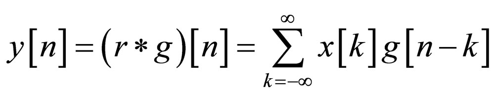
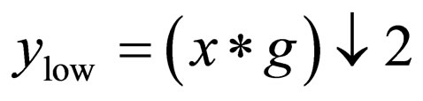
The DWT of an image x is calculated by passing it through a series of filters. First the samples are passed through a low pass filter with impulse response g resulting in a convolution of the two:
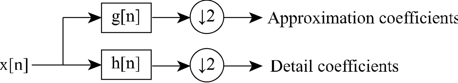
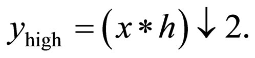
The image is also decomposed simultaneously using a high-pass filter h. The outputs give the detail coefficients (from the high-pass filter) and approximation coefficients (from the low-pass filter). It is important that the two
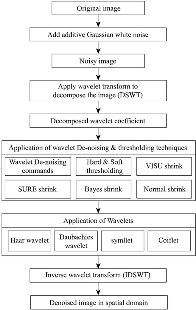
Figure 1. Block diagram of denoising using wavelet transformation and thresholding techniques.
filters are related to each other and they are known as a quadrature mirror filter. However, since half the frequencies of the signal have now been removed, half the samples can be discarded according to Nyquist’s rule. The filter outputs are then down sampled by 2: [9,10]
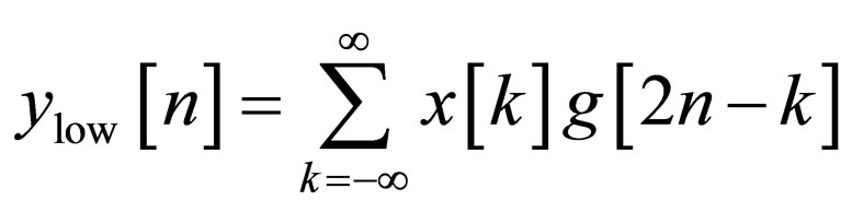
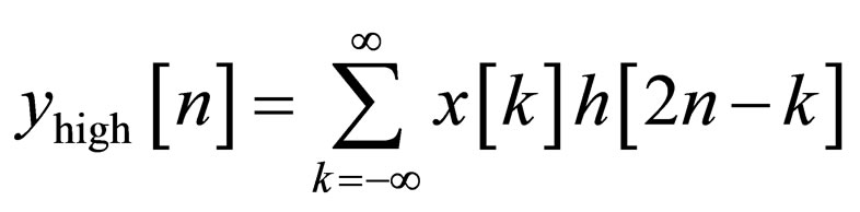
This decomposition has halved the time resolution, since only half of each filter output characterizes the signal. However, each output has half the frequency band of the input, so the frequency resolution has been doubled. This is in keeping with the Heisenberg uncertainty principle.
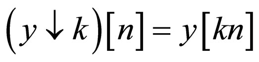
With the down sampling operator ↓ the above summation can be written more concisely.
The Discrete Wavelet Transform provides sufficient information both for analysis and reconstruction of the original signal, with a reduction in the computation time.
Sub-Band Coding
Sub-band coding is a method for calculating the Discrete Wavelet Transform. The whole sub-band process consists of a filter bank, and filters of different cut-off frequencies are used to analyze the signal at different scales.
The procedure starts by passing the signal through a half band high-pass filter and a half band low-pass filter. A half band low-pass filter eliminates exactly half the frequencies from the low end of the frequency scale. For example, if a signal has a maximum of 1000 Hz component, then half band low-pass filter removes all the frequencies above 500 Hz. The filtered signal is then down sampled, meaning some sample of the signal is removed. Then the resultant signal from the down sampled half band low-pass filter is then processed in the same way again. This process will produce sets of wavelet transform coefficients that can be used to reconstruct the signal. An example of this process is illustrated in Figure 2. The resolution of the signal is changed by filtering operations, and the scale is changed by down sampling operations. Down sampling a signal corresponds to reducing the sampling rate, which is equivalent to removing some of the samples of the signal.
Where, cAx is the approximation coefficients at decomposition level x, cDx is the detail coefficients at decomposition level x. S is the original signal. From Figure 2, you can see the original signal is broken down into different levels of decomposition. In the above case, it is a 3-level decomposition. Every time the newly scaled wavelet is applied to the signal, the information captured by the coefficients remains stored at that level. Thus the remaining information contains the higher frequencies of the signal, if the scaling factor decreases.
2.2. Stationary Wavelet Transform
The Stationary wavelet transform (SWT) is similar to the DWT except the signal is never sub-sampled and instead the filters are up sampled at each level of decomposition.
Each level’s filters are up-sampled versions of the previous as shown in Figure 3.
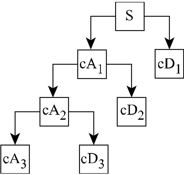
Figure 2. Wavelet decomposition tree.
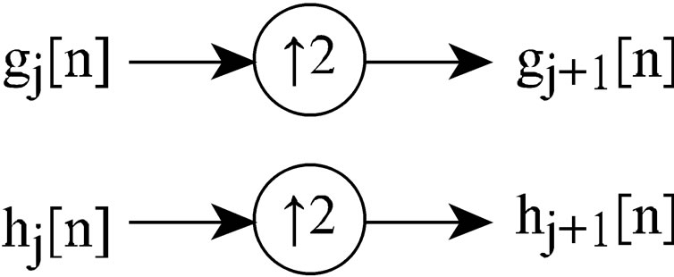
Figure 3. SWT filters.
The SWT is an inherent redundant scheme, as each set of coefficients contains the same number of samples as the input. So for a decomposition of N levels, there is a redundancy of 2N.
Figure 4 shows the decomposition of Discrete and Stationary wavelet transform. The Discrete Wavelet Transform (DWT) [11,12] is the simplest way to implement MRA. It necessitates a decimation by a factor 2N, where N stands for the level of decomposition, of the transformed signal at each stage of the decomposition. As a result, DWT is not translation invariant which leads to block artifacts and aliasing during the fusion process between the wavelet coefficients. For this reason, we use the Stationary Wavelet Transform (SWT) (Holschneider, 1988). For the SWT scheme the output signals at each stage are redundant because there is no signal downsampling; insertion of zeros between taps of the filters are used instead of decimation. Figure 5 shows the decomposition of an image using SWT at level 1.
3. Thresholding Techniques
Thresholding [13,14] is a simple non-linear technique, which operates on one wavelet coefficient at a time. In its most basic form, each coefficient which is smaller than threshold, set to zero, otherwise, it is kept or modified. The small co-efficient are dominated by noise, while coefficient with large absolute value carry more signal information than noise. Replacing noise co-efficient (small coefficients below a certain threshold value) by zero and an inverse wavelet transform may lead to a reconstruction that has lesser noise. This thresholding idea is based on the following:
1) The de-correlating property of wavelet transform creates a sparse signal. Most untouched coefficient is zero or close to zero.
2) Noise is spread out equally along all co-efficient.
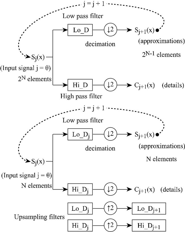
Figure 4. Decomposition of a 1-D signal using DWT (top) and SWT (bottom).

Figure 5. Decomposition using SWT at level 1.
3) The noise level is not too high so that one can distinguish the signal wavelet coefficients from binary ones.
This method is an effective and thresholding is simple and efficient method for noise reduction.
3.1. Hard Thresholding
One of the most attractive features of wavelet thresholding is that, for the type of random noise frequently encountered, in signal transmission, it is possible to automatically choose a threshold for denosing without any prior knowledge of the signal.
By choosing a threshold that is significantly large, and multiplying with the standard deviation of the random noise, it is possible to remove most of the noise by thresholding the wavelets transform coefficients. This process is known as hard thresholding.
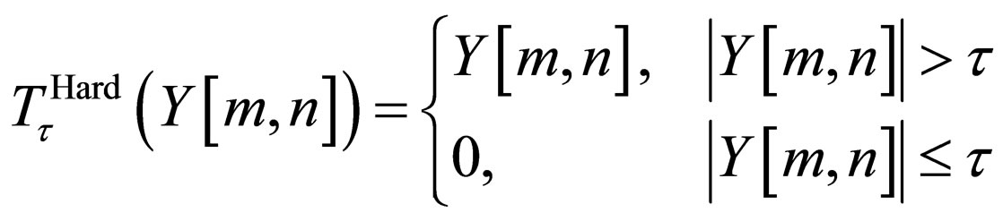
where, t is the threshold value.
From Figure 6, we can see that hard thresholding can create discontinuities, and thus greatly exaggerates small differences in the transform value whose magnitudes are near the threshold value t. If the value is only slightly less than t, then this value is set equal to zero, while a value whose magnitude is only slightly greater than t is left unchanged. Therefore, hard thresholding is not suitable for most noise removal. Figure 7 shows Hard thresholding uing dB5 wavelet.
3.2. Soft Thresholding
With a slight modification to the hard thresholding approach, a method known as soft thresholding can be created as shown in Figure 8.
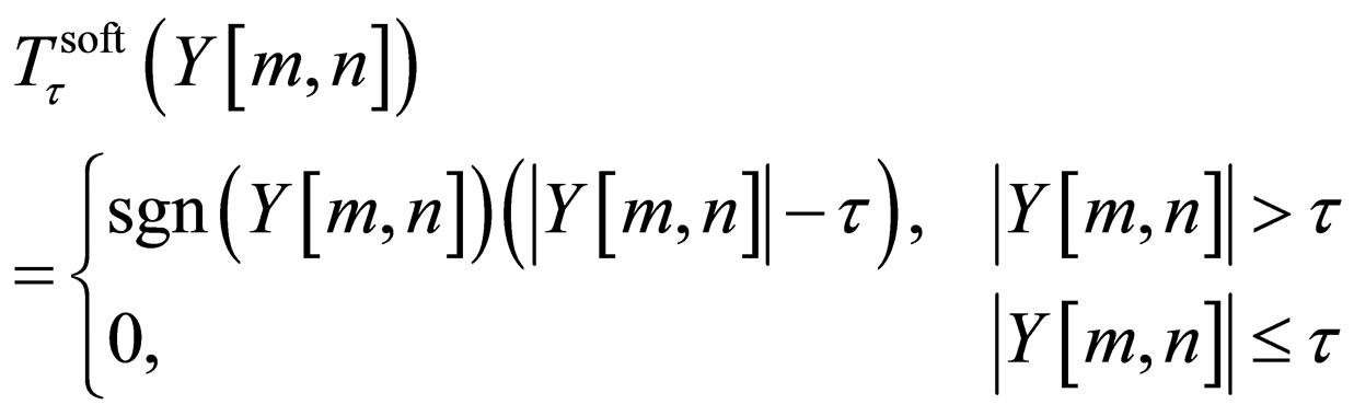
where, T is the threshold value.
From Figure 9, the original image had more noise in
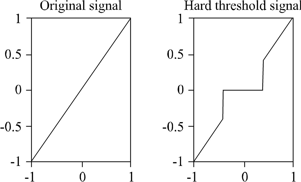
Figure 6. Illustration of hard thresholding, t = 0.4.
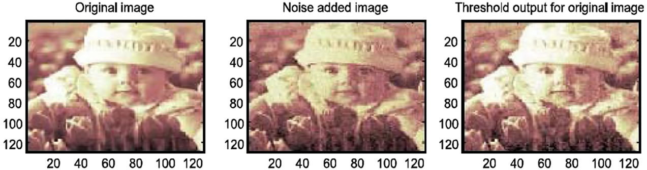
Figure 7. Hard thresholding using dB5 wavelet.
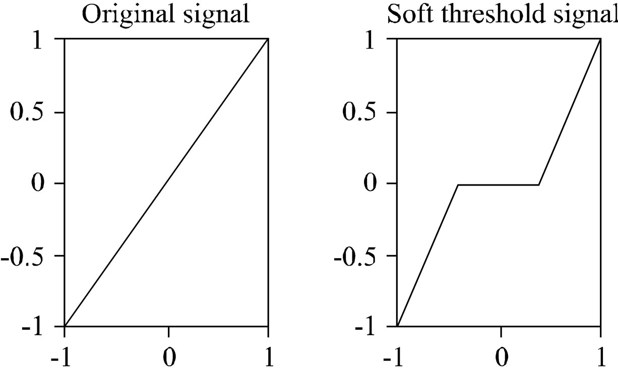
Figure 8. Illustration of Soft thresholding, with threshold t = 0.4.
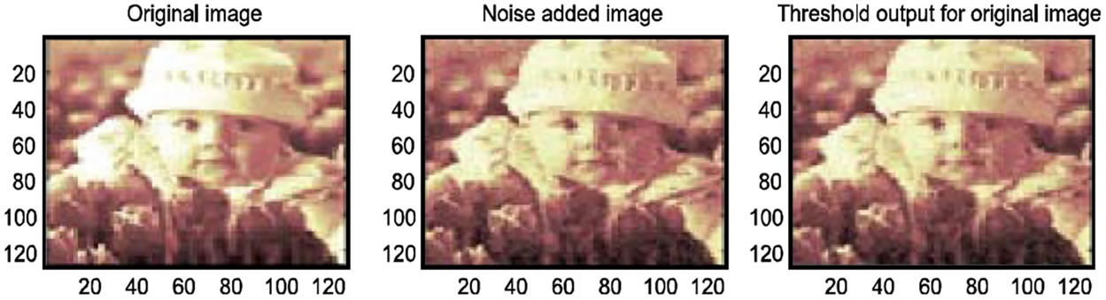
Figure 9. Soft thresholding using db5 wavelet.
the bottom half compared to the top half. Since soft thresholding is a global operation, in the sense the entire image is used for the denosing process, it cannot concentrate on just the lower half of the image. But, if the denoised image has to be processed again, then the top half of the image would be over processed, and defects, such as blurring, can be introduced. Some original details of the image is removed along with the noise. This is because the noise obscured most of the small magnitude values that result from the original signal. Consequently, when thresholding is applied, it removes many of the transform values of the original signal, which are needed for accurate approximation. To overcome this problem wavelet shrinkages are used.
3.3. Shrinkages
• 3.3.1. VISU Shrink
• VisuShrink is thresholding by applying the universal threshold proposed by Donoho and Johnstone.
• This threshold is given by 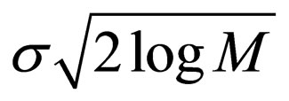
where σ is the noise variance and M is the number of pixels in the image.
• For denoising images, VisuShrink is found to yield an overly smoothed estimate.
• 3.3.2. SURE Shrink
• SURE Shrink [15] is a thresholding applied to subband adaptively.
• It is based on Stein’s Unbiased Risk Estimator (SURE), a method for estimating the loss in an unbiased fashion.
• Let wavelet coefficients in the jth sub-band be {Xi: i = 1, ∙∙∙, d}
• For the soft threshold estimator 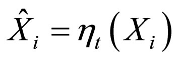
we have
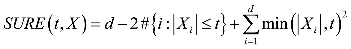
• Select threshold tS by
• 3.3.3. BAYES Shrink
• Bayes Shrink is an adaptive data-driven threshold for image de-noising via wavelet soft-thresholding.
• We assume generalized Gaussian distribution (GGD) for the wavelet coefficients in each detail sub-band.
• We then try to find the threshold T which minimizes the Bayesian Risk.
3.4. Experimental Results
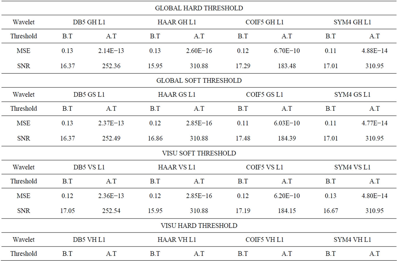
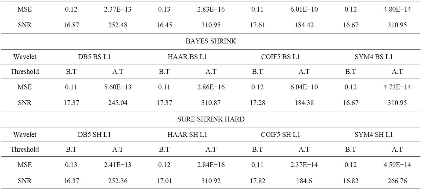
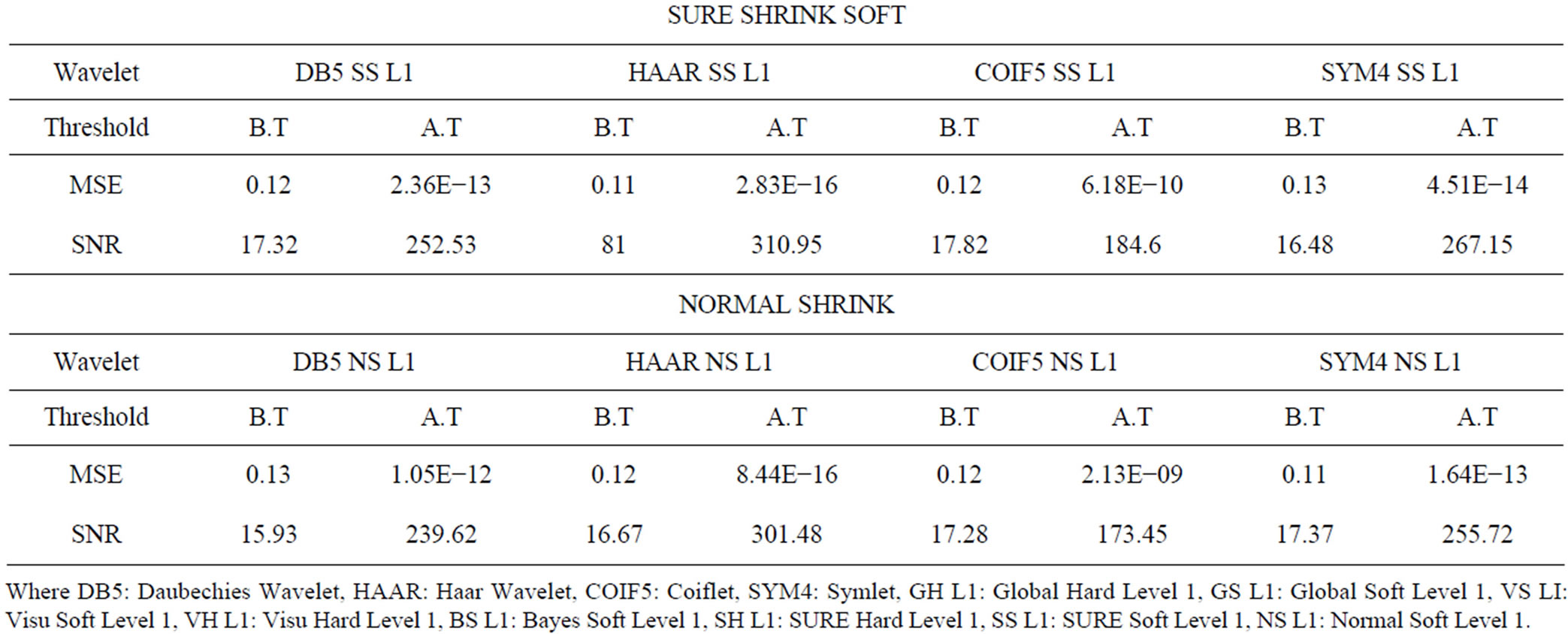
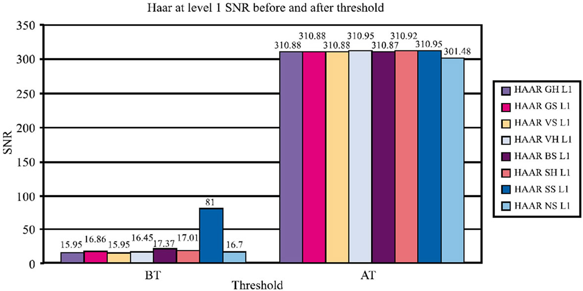
Figure 10. Graph for Haar at level 1 for SNR before & after thresholding.
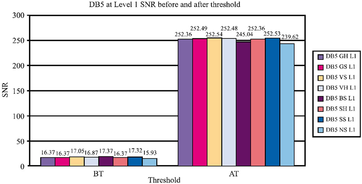
Figure 11. Graph for DB5 at level 1 for SNR before and after thresholding.
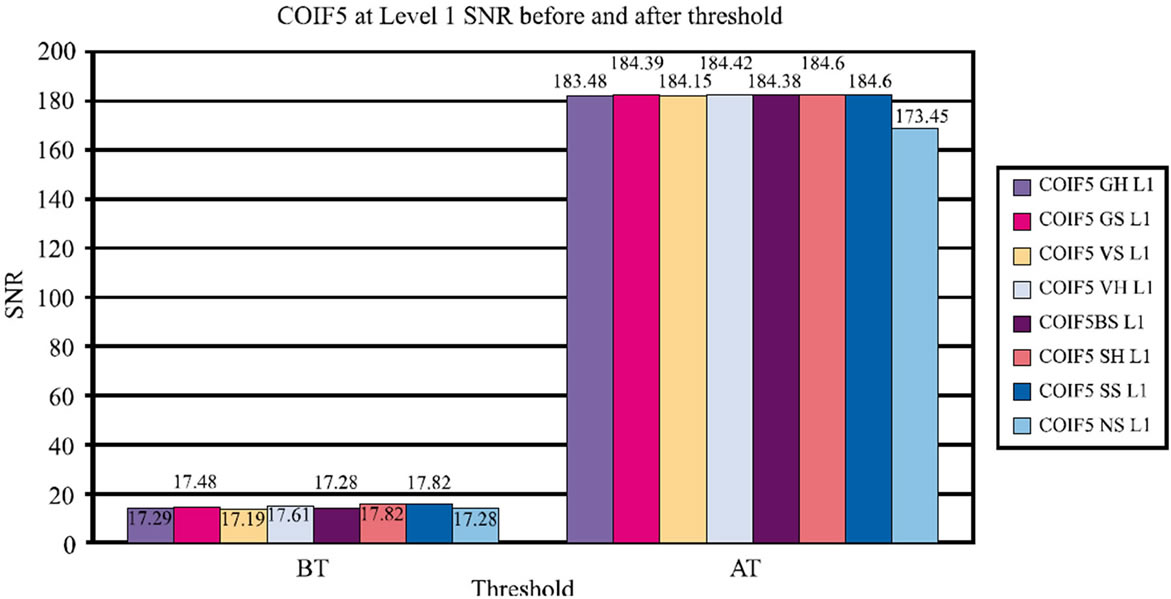
Figure 12. Graph for coiflet 5 at level 1 for SNR before & threshold
Comparison of SNR before and after thresholding for various wavelets at level 1 is shown in Figures 10-13. The Figure 14 shows image outputs for dB5 at level 1 for global soft thresholding.
3.5. Conclusion
DWT is translation varianopusion process between the wavelet co-efficient, where as DSWT is Translation Invariant. In DSWT artifacts and aliasing are less than compared to DWT. This is the reason, why DSWT is preferred over DWT. We have applied Additive White Gaussian Noise to an original image (kid), then DSWT is applied to get decomposed wavelet co-efficients to which various threshold techniques are applied for different wavelets. Inverse DSWT is applied to get reconstructed denoised image. In this paper, we have compared different wavelets such as Daubachies, Haar, Coiflet, Symlet with various threshold techniques such as default global hard and soft, VISU shrink soft and hard, Bayes shrink soft and Hard, SURE shrink soft and hard and Normal shrink and measured the parameters such as Mean Square Error (MSE) and Signal-to-Noise Ratio (SNR). After comparison, it is found that MSE for HAAR global hard wavelet threshold is the least among all. SNR for HAAR SURE shrink soft level 1 is the maximum and the best among all.
3.6. Future Scope
Nonetheless, there is always room for improvement. Multiwavelets are relatively a new subject of study. Most
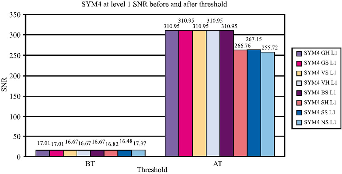
Figure 13. Graph for symlet 4 at level 1 for SNR before & after thresholding.
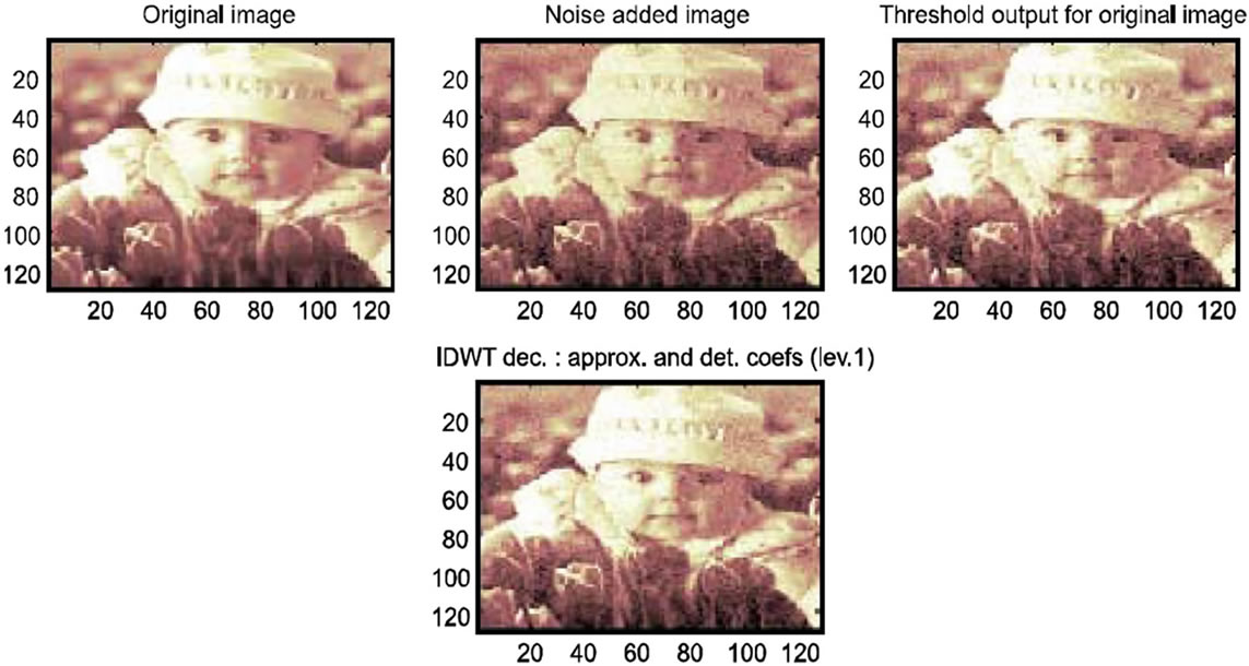
Figure 14. Image outputs for dB5 at level 1 for global soft thresholding.
current filters available have two, three or fourth order of approximation. Future construction methods may add even higher order of approximation, while preserving the desirable features of current methods. It most likely result in multi-filters that perform even better in image denoising & compression applications. Moreover the multiwavelet systems available presently have the multiscaling and multiwavelet coefficients which are 2 × 2 matrices. There is a possibility that in future many more multiwavelet systems might be developed with matrix coefficients with higher order, which could provide even beter results in the field of image denoising & compression.
REFERENCES
- S. Mallat, “A Wavelet Tour of Signal Processing,” Cambridge Univiversity Press, New York, 1999.
- V. Strela and A. T. Walden, “Signal and Image Denoising via Wavelet Thresholding: Orthogonal and Biorthogonal, Scalar and Multiple Wavelet Transforms,” Statistic Section Technical Report TR-98-01, Department of Mathematics, Imperial College, London, 1998.
- D. L. Donoho and I. M. Johnstone, “Denoising by Soft Thresholding,” IEEE Transactions on Information Theory, Vol. 41, No. 3, 1995, pp. 613-627. doi:10.1109/18.382009
- S. G. Chang, B. Yu and M. Vattereli, “Wavelet Thresholding for Multiple Noisy Image Copies,” IEEE Transactions on Image Processing, Vol. 9, No. 9, 2000, pp.1631-1635. doi:10.1109/83.862646
- D. L. Donoho and I. M. Johnstone, “Ideal Spatial Adaptation by Wavelet Shrinkage,” Biometrika, Vol. 81, No. 3, 1994, pp. 425-455. doi:10.1093/biomet/81.3.425
- A. M. L. Lanzolla, G. Andria, F. Attivissimo, G. Cavone, M. Spadavecchia and T. Magli, “Denoising Filter to Improve the Quality of CT Images,” Proceedings of IEEE Conference on Instrumentation and Measurement Technology, Singapore City, 5-7 May 2009, pp. 947-950.
- S. Ruikar, Andria and D. D. Doye, “Image Denoising Using Wavelet Transform,” International Conference on Mechanical and Electrical Technology (ICMET 2010), Singapore City, 10-12 September 2010, pp. 509-515.
- I. Daubechies, “The Wavelet Transform, Time-Frequency Localization and Signal Analysis,” IEEE Transaction on Information Theory, Vol. 36, No. 5, 1990, pp. 961-1005.
- J. Portilla, V. Strela, M. Wainwright and E. Simoncelli, “Image Denoising Using Gaussian Scale Mixtures in the Wavelet Domain,” IEEE Transactions on Image Processing, Vol. 12, No. 11, 2003, pp. 1338-1351. doi:10.1109/TIP.2003.818640
- J. Portilla and E. P. Simoncelli, “Adaptive Wiener Denoising Using a Gaussian Scale Mixture Model in the Wavelet Domain,” IEEE International Conference on Image Process (ICIP), Vol. 2, 2001, pp. 37-40.
- S. G. Chang, B. Yu and M. Vetterli, “Adaptive Wavelet Thresholding for Image Denoising and Compression,” IEEE Transactions on Image Processing, Vol. 9, No. 9, 2000, pp. 1532-1546.
- A. Pizurica, W. Philips, I. Lemahieu and M. Acheroy, “A Versatile Wavelet Domain Noise Filtration Technique for Medical Imaging,” IEEE Transactions on Medical Imaging, Vol. 22, No. 3, 2003, 323-331.
- M. K. Mihcak, I. Kozintsev, K. Ramchandran and P. Moulin, “Low-Complexity Image Denoising Based on Statistical Modelling of Wavelet Coefficients,” IEEE Signal Processing Letters, Vol. 6, No. 12, 1999, pp. 300-303. doi:10.1109/97.803428
- I. M. Johnstone and B. W. Silverman, “Wavelet Threshold Estimators for Data with Correlated Noise,” Journal of the Royal Statistical Society B, Vol. 59, No.2, 1997, pp. 319-351. doi:10.1111/1467-9868.00071
- F. Luisier, T. Blu and M. Unser, “A New SURE Approach to Image Denoising: Interscale Orthonormal Wavelet Thresholding,” IEEE Transactions on Image Processing, Vol. 16, No. 3, 2007, pp. 593-606. doi:10.1109/TIP.2007.891064