Agricultural Sciences
Vol.4 No.8A(2013), Article ID:35978,9 pages DOI:10.4236/as.2013.48A004
Integration of colour bathymetry, LiDAR and dGPS surveys for assessing fluvial changes after flood events in the Tagliamento River (Italy)
![]()
Department of Land, Environment, Agriculture and Forestry, University of Padua, Padua, Italy; *Corresponding Author: marioaristide.lenzi@unipd.it
Copyright © 2013 Johnny Moretto et al. This is an open access article distributed under the Creative Commons Attribution License, which permits unrestricted use, distribution, and reproduction in any medium, provided the original work is properly cited.
Received 16 May 2013; revised 17 June 2013; accepted 20 July 2013
Keywords: Erosion-Deposition Pattern; LiDAR Data; dGPS Survey; Colour Bathymetry; Floods; Gravel Bed Braided River; Tagliamento River
ABSTRACT
The estimation of underwater features of channel bed surfaces without the use of bathymetric sensors results in very high levels of uncertainty. A revised approach enabling an automatic extraction of the wet areas to create more accurate and detailed Digital Terrain Models (DTMs) is here presented. LiDAR-derived elevations of dry surfaces, water depths of wetted areas derived from aerial photos and a predictive depth-colour relationship were adopted. This methodology was applied at two different reaches of a northeastern Italian gravel-bed river (Tagliamento) before and after two flood events occurred in November and December 2010. In-channel dGPS survey points were performed taking different depth levels and different colour scales of the river bed. More than 10,473 control points were acquired, 1107 in 2010 and 9366 in 2011 respectively. A regression model that calculates channel depths using the correct intensity of three colour bands (RGB) was implemented. LiDAR and water depth points were merged and interpolated into DTMs which features an average error, for the wet areas, of ±14 cm. The different number of calibration points obtained for 2010 and 2011 showed that the bathymetric error is also sensitive to the number of acquired calibration points. The morphological evolution calculated through a difference of DTMs shows a prevalence of deposition and erosion areas into the wet areas.
1. INTRODUCTION
The study of river morphology and dynamics is essential to understanding the factors (natural and anthropic) determining sediment erosion, transport and deposition processes [1]. To better analyze the magnitude of different morphological adjustments occurring in river channels, precise quantitative approaches are needed. Threedimensional and high-resolution representations of river bed morphology have recently been used for detailed hydraulic modeling [2], for evaluating the impact of climate change [3], and for flood risk management [4]. The definition of hazardous areas also includes the assessment of erosion and deposition areas along the river corridor [5]. Different methods proved to be able to provide high-resolution Digital Elevation Models (DEMs) of fluvial systems. Recent studies on morphological channel changes have used passive remote sensing techniques such as digital image processing [6], digital photo grammetry [7], active sensors including Laser Imaging Detection and Ranging (LiDAR) [8], Terrestrial Laser Scanner [9] and acoustic methods [10]. The main problem related to the production of precise DEMs without using bathymetric sensors is due to the absorption of natural (solar) or artificial (LiDAR) electromagnetic radiation in the wetted channel. Only few tools have demonstrated to be able to provide an accurate and high-resolution measure of the bed surface elevation within wetted channels, also considering that survey precision decreases with the increase of the water depth. Bathymetric LiDAR sensors should be able to detect underwater bed surfaces. Nevertheless, they feature high costs, relatively low resolutions, and data quality comparable to photo grammetric techniques [11].
The survey of wetted areas can be thus approached using techniques based on the calibration of a depthreflectance relationship of images, which can be in greyscale [12], coloured [13,14] or multispectral [15]. All the solutions need a field survey, contemporary to the flight, to allow the availability of calibration depth points.
The present work proposes the implementation, on the Tagliamento River, of an optimized version of the [14] methodology. This approach consists of a calibration of a depth-colour model to estimate channel water depths. After a filtering process, based on the identification of erroneous depth values due mostly to reflection and sediments exposed, the bathymetric points for the wet areas and the LiDAR points for the dry areas will be merged to produce the final Hybrid Digital Terrain Models (HDTMs).
The specific objectives can be summarized as follows: 1) optimizing wet area extraction with a revised automatic methodology; 2) apply the [14] approach in a more complex braided river system; 3) evaluate limits and potentials of this procedure with attention to the factors influencing in a significant way the quality of final results.
2. STUDY AREA
2.1. Tagliamento River
The study was performed in the Tagliamento River, one of the last European rivers still maintaining a high degree of naturalness and representing an important biogeographical corridor with a strong longitudinal, lateral and vertical connectivity, high habitat heterogeneity, a characteristic sequence of geomorphic types and very high biodiversity [16].
The Tagliamento River is a gravel-bed river located in the Southern Alps in North-Eastern Italy (Friuli Venezia Giulia region). It originates at 1195 m a.s.l. and flows for 178 km to the north Adriatic Sea, thereby forming a link corridor between the Alps and the Mediterranean zones. Its drainage basin covers 2871 km2 (Figure 1). The catchment is limited by the Carnic Alps (North); by Piave, Livenza and Meduna basins to the West; and by Isonzo and Torre basins to the East. The river has a straight course in the upper part, while the most of its path is braided shifting to meandering in the lower part, where dykes have constrained the last 30 km (it features the characteristics of an artificial channel with a width of about 175 m). However, the upper reaches are more or less intact, thus the basic river processes, such as flooding, and sediment transport, take place under near-natural conditions.
The hydraulic regime of the Tagliamento River is characterized by an irregular discharge and a high sedimentation load; due to the climatic and geological condi-

Figure 1. The Tagliamento River catchment and Cornino and Flagogna sub-reaches.
tions of the upper part (annual precipitation can reach 3100 mm). The catchment is mainly mountainous and the slopes are very steep, leading to high peak flows and sediment loads in the central and lower part of the basin. The climatic characteristics of the catchment area result in a bi-modal pluvial flow regime. As all braided river channels, also the Tagliamento is characterized by a marked instability due to easily erodable banks, high sediment transport rates and considerable width of the valley [9]. This in turn leads to a frequent remodelling of the morphological elements. The large size of the floodplain and the rapid morphological variation are the main reasons accounting for the absence of a good stage-discharge relationship. In the present study, we refer to the water stage level recorded at the Venzone gauging Station (Figure 2).
2.2. Analyzed Sub-Reaches
The LiDAR survey and analysis were performed in two sub-reaches located near to the village of Forgaria nel Friuli, in Friuli, Venezia Giulia Region.
The upstream sub-reach (Figure 1), called “Cornino”, shows a predominant braided morphology, channels are separated by vegetated islands and gravel bars. The length is about 3 km and the active channel width ranges from a maximum of 1 km to a minimum of 700 m with a slope of around 0.35%. This sub-reach is characterized by a heterogeneous sediment size composition ranging from medium-fine sand to coarse gravel.
The lower, called Flagogna sub-reach has a predominant wandering morphology with central bars and dead channels. As shown in the Figure 1, the main channel flows almost exclusively through the left bank and, as in Cornino sub-reach, there is a large number of longitudinal and lateral bars and river islands mostly located in the right side. The length is about 3.5 km and the active channel width is between 300 and 800 m, with a slope of around 0.30%.
3. MATERIALS AND METHODS
The methodological approach of this paper has the principal aim of producing Digital Terrain Models (DTMs) derived from LiDAR data, acquired contemporary to aerial photos and a dGPS survey, with the highest accuracy possible also in the wet areas. To create these
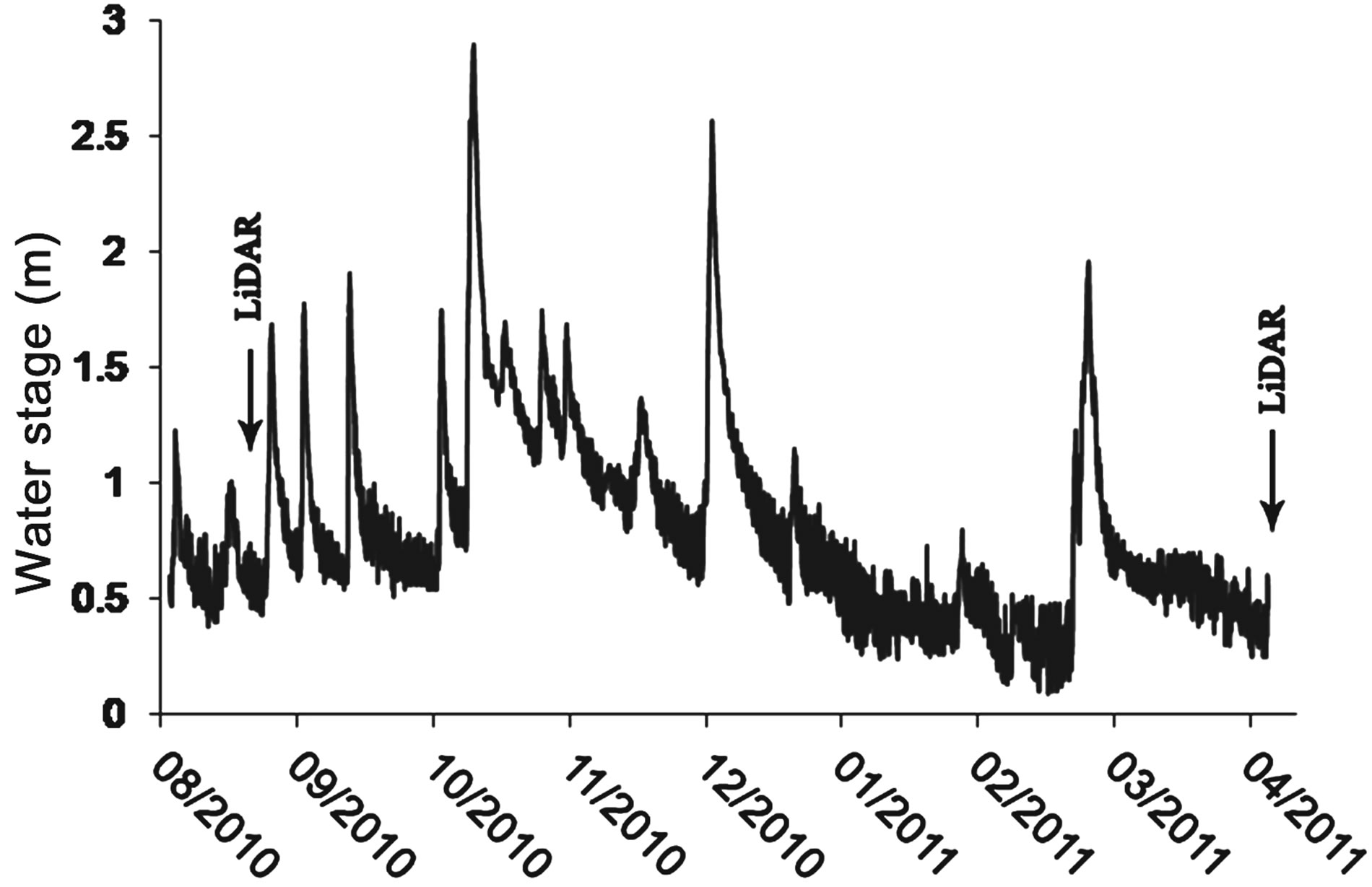
Figure 2. Hourly water level recorded at the Venzone hydrometric station between the two LiDAR surveys.
elevation models we have used the same colour bathymetry method used by [14] but with an optimization concerning the wet area digitalization process. The procedure to estimate the water depth provides a statistical regression between water depth (Dph) and red, green and blue intensity values (R, G and B). The details of this optimization and the principal steps of the colour bathymetry process are reported in the sub-headings below.
3.1. Data Acquisition
Two LiDAR surveys were carried out: the first in August 2010 by Blom GCR Spa through an OPTECH ALTM Gemini sensor and the second in April 2011 by OGS Company through a RIEGL LMS-Q560 sensor (flying height ~850 m) after the significant floods Registered on November and December 2010 (Figure 2). For each LiDAR survey a point density able to generate digital terrain models with 0.5 m of resolution (at least 2 ground points per square meter) was required. The average vertical error of the LiDAR has been evaluated trough dGPS points on the final elevation model. LiDAR data were taken together with a series of RGB aerial photos with 0.15 m pixel resolution. The survey was carried out with the best weather conditions and low hydraulic channel levels. In-channel dGPS points acquisition was performed, taking different depth levels in a wide range of morphological units. Overall, 1107 points in 2010 and 9366 points in 2011 were acquired. Finally, for each subreach, control points were surveyed through dGPS (dGPS average vertical error ±0.025 m). Important is to note that the dGPS capture have been performed contemporary with the LiDAR acquisition to avoid additional stochastic components.
3.2. Automatic Wet Area Extraction
A revised approach proposed by [17], regarding the determination of the wet areas through a combination of a canopy surface model (CSM; difference between digital surface model and digital terrain model) and the intensity of the LiDAR signal (Figure 3), was carried out. To estimate wet areas we have used a combination of LiDAR intensity, CSM and a detrended DTM (without slope). The purpose of each component was: 1) to divide the zone with very low intensity (as water and vegetation) from the zone with high intensity (as gravel) as shown in Figure 3; 2) to divide vegetation from the water; 3) to divide artificial pool-lakes and channels (with different “altitude elevation level”) from the river channels. Wet are as were defined with a LiDAR intensity lower than 55 (as in [17]) and a CSM elevation lower than 0.5 m. The “natural wet area” from artificial pool-lakes or channels on the detrended DTM was extracted with a “threshold elevation” in function of the study area. This as-
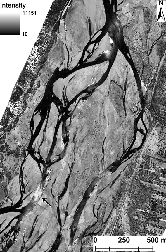
Figure 3. LiDAR intensity raster of Cornino sub-reach in 2011. The arrow indicates an area with anomalous intensity values.
sumption was made because the fluvial channels of the Tagliamen to River are always below artificial (poollakes) wet areas.
Elaborations have been performed in ArcGIS 10® using a developed macro-utility, starting from LiDAR intensity, CSM and detrended DTM rasters. The results can be viewed as an output representing, with a shape file, the wet area. This approach, applied to a large river with braided morphology such as the Tagliamento, significantly decreases the time employed for extracting the wet areas of the active natural channel. In addition, the resulting shape file can be easily modified, in the case of anomalous intensity values that produce uncertainty detection of the real wet areas (see arrow in the Figure 3).
3.3. Indirect Estimates of the Water Level and Dataset Preparing
Along the edges of the “wet area” shape polygon, reliable LiDAR points able to represent the water surface elevation (Zwl) in our inference zone were selected. The correspondent intensity of the colour bands and Zwl were added to the points acquired in the wetted areas (dGPS wet-area survey) obtaining a shape file of points containing five fields (in addition to the spatial coordinates X and Y): the intensity of the three colour bands, Red (R), Green (G), Blue (B), the elevation of the channel bed (Zwet) and Zwl. Finally, the channel depth was calculated as Dph = Zwl – Zwet.
3.4. Bathymetric Model Determination
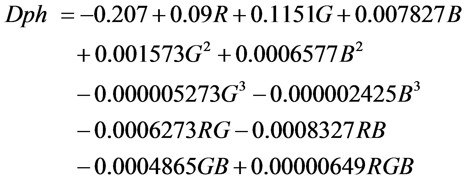
As in [14], an empirical depth linear model testing all the colour bands, the possible interaction of variables and the square and cubic terms was tested:
 (1)
(1)
where α and βx are the calibration coefficients in the depth-colour regression. In this model, the significance of each component was tested, deleting the statistically negative values.
The statistical regressions have been performed in R® environment using the 80% of the calibration points and two methods: the traditional regression method based on the statistical significance, tested on each variable (p-value < 0.05), and the AICc index [18]. The model featuring the lowest error (tested with the 20% of the dGPS points not used to calibrate the model) was used to build the “Raw channel Depth raster” (RDph).
3.5. Hybrid DTM Creation and Validation
The best bathymetric model was applied to the georeferenced photos (raster calculator) to determine the RDph. The RDph was then transformed into points (density of around 2 points/m2) and was filtered in order to delete incorrect or suspicious points, mainly due to sunlight reflections, turbulence, and elements (wood or sediment) above the water surface.
The methodology proposed in [14] to filter possible incorrect points providing a detection of slope changes in neighbouring pixels, was applied. Indeed, in occasion of very strong slope changes between neighboring pixels, a potential error of depth estimation is present. The corresponding Zwl was added to the corrected points (Dph model) to obtain, for each point, the estimated elevation of the river bed (Zwet = Dph + Zwl). Hybrid DTMs (HDTM) were built up with the natural neighbor interpolator, integrating Zdry points (by LiDAR) in the dry areas and Zwet points (by colour bathymetry) in the wet areas.
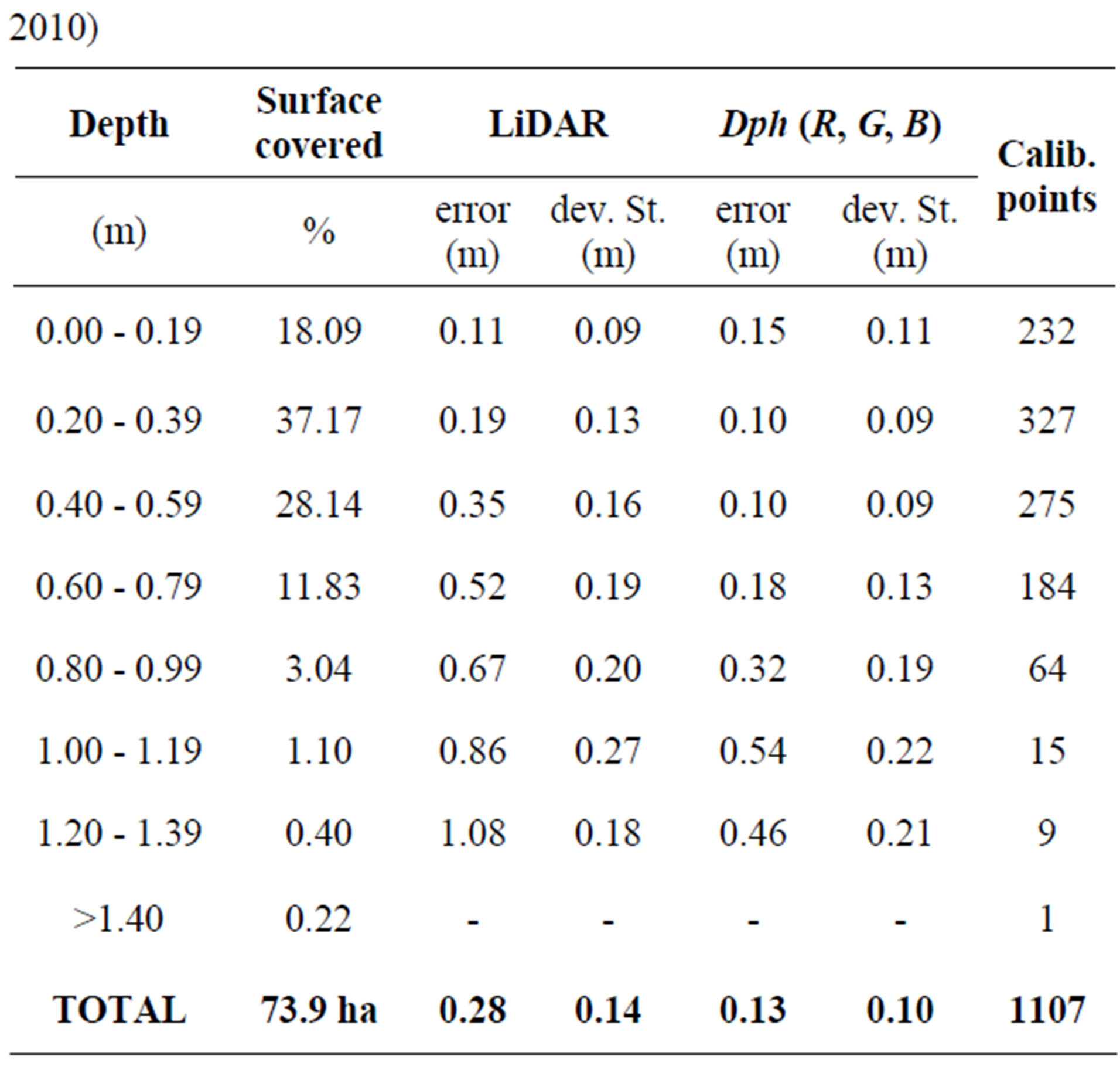
The final step was the validation of the HDTM models which was carried out by comparison with dGPS surveys (1107 points in 2010 and 9366 points in 2011). The accuracy of the hybrid DTMs was estimated for wet areas considering colour bathymetry errors at different water stage levels grouped in classes incremented of 20 cm (see Table 1).
4. RESULTS
4.1. Wet Area Extraction
The revised method to automatically extract wet areas has demonstrated a very good performance as reported in Figure 4(a). The strong difference in LiDAR intensity
 2010)
2010)  2011)
2011)
Table 1.Error analysis of LiDAR and depth-colour models at different water stages for 2010 and 2011.
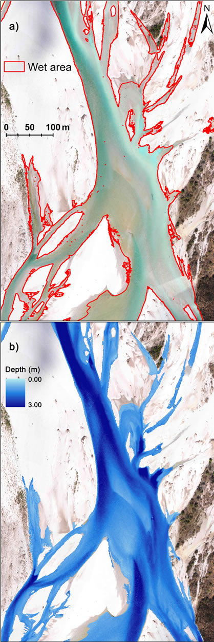
Figure 4. Automatic wet area extraction (a) and colour bathymetry application (b) of Cornino sub-reach in 2011.
between water and gravel has allowed to achieve a good edge definition. The associated rasters (CSM, and detrended DTM) have allowed to delete the dry are as featuring a similar intensity. Therefore the resulting shape files can be used to divide the wet from the dry areas.
4.2. Colour Bathymetry Models
The statistical regressions performed with the two different approaches (traditional regression and AICc) have produced two bathymetric models for each inter-flood period.
For 2010, both statistical regression methods have demonstrated that all the colour bands are significantly correlated with the water depth. In addition to the presence of correlation between the colour bands and a nonlinear regression, we have also found that the interactions and the square and cubic terms are all significant. The traditional regression methods have demonstrated a little better performance than the AICc:
 (2)
(2)
where Dph is the estimated water depth and R, G and B the red, green and blue intensity bands, respectively. This model, if compared with the final HDTM, estimates the wet area with ±0.13 m of weighted error (with the area of influence of each band on the water depth) and a standard deviation error of ±0.10 m (Table 1).
Similar results are featured for 2011, but in this case the AICc method has demonstrated the best results:
 (3)
(3)
All the terms in these models are statistically significant; a small scale (Figure 4(b)) and two large scales (Figures 5 and 6) examples regarding the results of the model application are shown.
From a general point of view the model seems to be able to produce a good water depth estimation if compared to the aerial photos, as in Figure 4(a).
This model, compared with the final HDTM, estimates the wet area with ±0.15 m of weighted error (with the area of influence of each band on the water depth) and a standard deviation of ±0.11 m (Table 1).
5. DISCUSSION
The different water depth errors estimated from LiDAR and from the proposed colour bathymetric approach have been compared to the 2010 and 2011 surveys and reported on Table 1.
The results confirm that the LiDAR signal features an average error greater than ±0.20 m already after ~0.20 m of water depth and greater than ±0.50 m after ~0.60 m of depth. These underestimations are mainly due to the
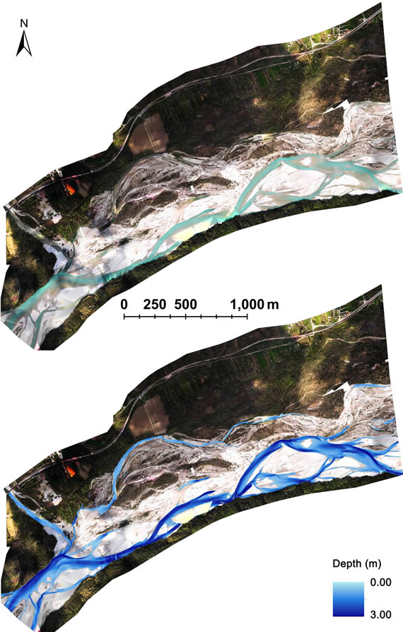
Figure 5. Bathymetric model application on all wet areas of Cornino 2011 sub-reach.
signal adsorption and, in some cases (where the channel is not perpendicular to the laser beams); to the low angle of incidence that causes an underestimate of the channel depth and an overestimate of the bank full width [19].
In the case of braided morphologies, such as in the Tagliamento River, if the wet areas are excluded in the estimation of erosion and deposition volumes, results far from the real change can be obtained.
On the other hand, the applied colour bathymetry is able to produce depth estimates with an average error lower than ±0.20 m until ~0.80 m for the 2010 and until ~1.40 m for the 2011. These depths represent, for the 2010 and for the 2011 respectively, the 95.2% and 96.2% of the total wet area.
The average water level depths in the Tagliamento sub-reaches were a little higher during April 2011 surveys (LiDAR, bathymetry and dGPS) than August 2010. Hence, a greater number of dGPS calibration points were acquired in 2011 (9366 values), particularly concentrated (Table 1) in the depth layer between 0.40 m and 1.20 m (7372 calibration points representing the 81.3% of wet
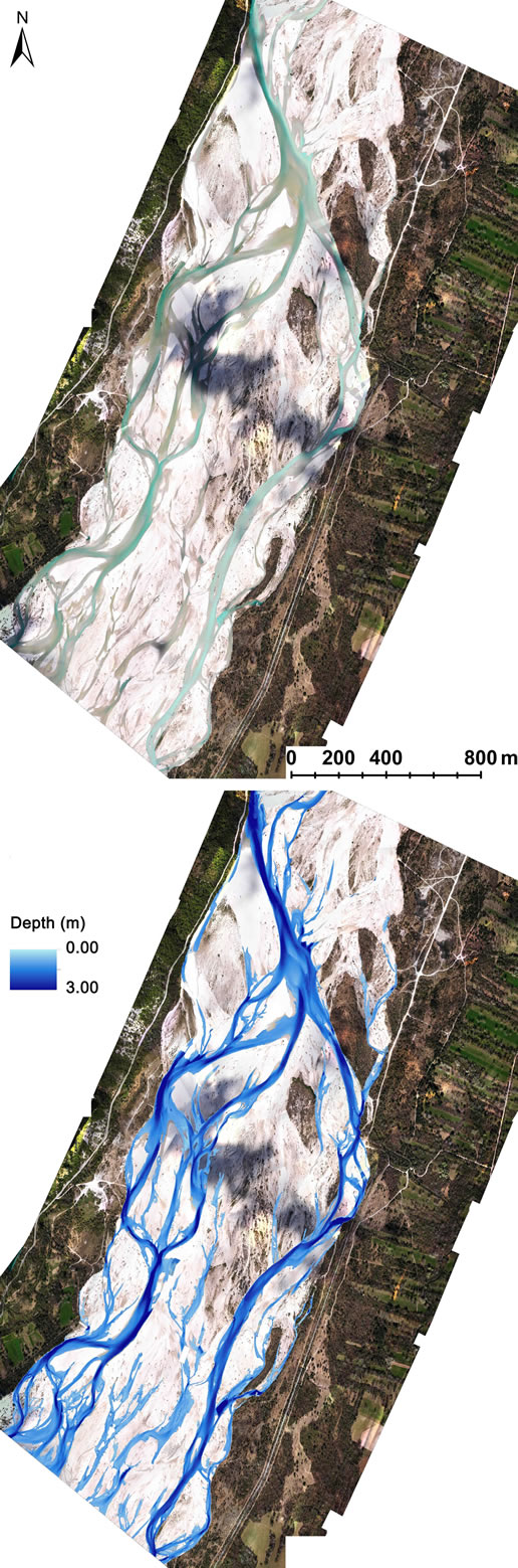
Figure 6. Bathymetric model application on all wet areas of Flagogna 2011 sub-reach.
surface covered).
More the depth increases, greater is the light adsorbed as described by [20], raising the variability of R, G and B colour bands. This greater variability decreases the quality of the results of the colour models. Despite this decrease in quality, an adequate number of calibration points allow to reach an acceptable error (similar to the LiDAR) for more than 95% of the wet area (in our case). The 64 calibration points included in a depth around 0.80 - 1.00 m, seem to be not enough to produce an error lower than ±0.20 m (see Table 1, 2010 survey error values). The 341 dGPS control points seem to be also not enough, in the case of the 2011 survey, for estimating depth higher than 1.40 m. Therefore, a preliminary analysis to know both, the range of depths and the percentage of wet surface covered in the study reach is required. In this way, we can decide, thanks also to the help of the Table 1, the minimum number of dGPS points allowing an acceptable error for the major part of the wet area.
Other important rules to produce a reliable colour bathymetry are: 1) commissioning LiDAR and aerial photo surveys with the lowest water depth and suspended sediment load; 2) flight time around midday, to avoid shadows which can introduce more errors on the colour models; 3) perfect photo-georeferenziaton; 4) good water level estimation. The difference of DEM (DoD), of Cornino and Flagogna sub-reaches, derived from the 2011 and 2010 HDTM obtained by merging LiDAR data for the dry areas and colour bathymetry data for the wet areas, are shown in Figures 7 and 8.
These changes are due to the flood events of November-December 2010 (Figure 2). The most part of the variations have occurred in the wet areas; similar results have been highlighted in [14]. Thanks to the colour bathymetry we can reach a “reliable” bedform representation in all the study area.
Following the [14] methodology and the optimization of the wet area extraction (automatic extraction) reported in this paper we have created the basis for more meaningful quantifications of erosion and deposition volumes, sediment budgets and further applications of 2D or 3D modelling, useful for management purposes.
6. CONCLUSIONS
The proposed methodology allows the production of high-resolution DTMs of wetted areas with an associated uncertainty which is comparable to LiDAR data. The bathymetric model calibration requires only a dGPS survey in the wet areas contemporaneous to the aerial image acquisition. The statistical analyses have demonstrated that all the three colour bands (R, G, B) significantly relate to water depth.
The different number of calibration points between 2010 (1107 values) and 2011 (9366 values) has shown
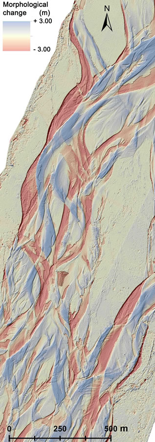
Figure 7. Difference of DEMs (DoD) of Cornino sub-reach.

Figure 8. Difference of DEMs (DoD) of Flagogna sub-reach.
that the error of the colour bathymetry is significantly related also to the number of calibration points acquired. Indeed, the applied colour bathymetry is able to produce depth estimates with an average error lower than ±0.20 m until ~0.80 m for the 2010, but until ~1.40 m for the 2011.
A preliminary analysis to know both, the range of depths and the percentage of the wet surface covered in the study reach is required to decide the minimum number of dGPS points that allows an acceptable error on the wet area.
The raster of difference (DoD) highlights the consequences of the flood events of November-December 2010, indicating that deposition and erosion areas are more concentrated into the wet areas. In the analysis of braided morphologies, such as in the case of the Tagliamento River, the calculation of uncorrected estimations of change in those areas can lead to volumetric results far from the real values.
The results of this study can be a valuable support to generate precise elevation models, also for the wet areas, that can be useful to evaluate erosion-deposition patterns, to improve sediment budget calculation, numerical modeling and to develop more effective river management strategies. The previous explained automatic extraction of the flowing channel will be important in the decrease of the time consumed for the data elaborations.
7. ACKNOWLEDGEMENTS
This research was founded by the University of Padua Strategic Research Project PRST08001, “GEORISKS, Geological, morphological and hydrological processes: monitoring, modelling and impact in NorthEastern Italy”, Research Unit STPD08RWBY-004; the Italian National Research Project PRIN20104ALME4-ITSedErosion: “National network for monitoring, modeling and sustainable management of erosion processes in agricultural land and hilly-mountainous area”; and The EU SedAlp Project: “Sediment management in Alpine basis: Integrating sediment continuum, risk mitigation and hydropower”, 83-4-3-AT, in the framework of the European Territorial Cooperation Programme Alpine Space 2007-2013.
REFERENCES
- Moretto, J., Rigon, E., Mao, L., Picco, L., Delai, F. and Lenzi, M.A. (2013) Channel adjustments and island dynamics in the Brenta River (Italy) over the last 30 years. River Research and Applications, in Press.
- Rumsby, B.T., Brasington, J., Langham, J.A., McLelland, S.J., Middleton R. and Rollingson G. (2008) Monitoring and modelling particle and reach-scale morphological change in gravel-bed rivers: Applications and challenges. Geomorphology, 93, 40-54. doi:10.1016/j.geomorph.2006.12.017
- Rumsby, B.T. and Macklin, M.G. (1994) Channel and floodplain response to recent abrupt climate change: The tyne basin, Northern England. Earth Surface Processes and Landforms, 19, 499-515. doi:10.1002/esp.3290190603
- Macklin, M.G. and Rumsby, B.T. (2007) Changing climate and extreme floods in the British uplands. Transactions of the Institute of British Geographers, 32, 168-186.
- Lane, S.N., Tayefi, V., Reid, S.C., Yu, D. and Hardy, R.J. (2007) Interactions between sediment delivery, channel change, climate change and flood risk in a temperate upland environment. Earth Surface Processes and Landforms, 32, 429-446. doi:10.1002/esp.1404
- Legleiter, C.J. and Roberts, D.A. (2009) A forward image model for passive optical remote sensing of river bathymetry. Remote Sensing of Environment, 113, 1025-1045. doi:10.1016/j.rse.2009.01.018
- Lane S.N., Widdison P. E., Thomas R.E., Ashworth P.J., Best J.L., Lunt I.A., Sambrook Smith, G.H. and Simpson, C.J. (2010) Quantification of braided river channel change using archival digital image analysis. Earth Surface Processes and Landforms, 35, 971-985. doi:10.1002/esp.2015
- Hicks, D.M. (2012) Remotely sensed topographic change in gravel riverbeds with flowing channels. In: Church, M., Biron, P.M. and Roy, A.G. Eds., Gravel-Bed Rivers: Processes, Tool, Environments, Wiley-Blackwell, 303-314. doi:10.1002/9781119952497.ch23
- Picco, L., Mao, L., Cavalli, E., Buzzi, E., Rigon, E., Moretto, J., Delai, F., Ravazzolo, D. and Lenzi, M.A. (2012) Using a Terrestrial Laser Scanner to assess the morphological dynamics of a gravel-bed river. IAHS-AISH Publication, Wallingford, 428-437.
- Rennie, C.D. (2012) Mapping water and sediment flux distributions in gravel-bed rivers using ADCPs. In: Church, M., Biron, P.M. and Roy, A.G. Eds., Gravel-Bed Rivers: Processes, Tool, Environments, Wiley-Blackwell, 342- 350.
- Hilldale, R.C. and Raff, D. (2008) Assessing the ability of airborne LiDAR to map river bathymetry. Earth Surface Processes and Landforms, 33, 773-783. doi:10.1002/esp.1575
- Winterbottom, S.J. and Gilvear, D.J. (1997) Quantification of channel bed morphology in gravel-bed rivers using airborne multispectral imagery and aerial photography. Regulated Rivers: Research and Management, 13, 489-499. doi:10.1002/(SICI)1099-1646(199711/12)13:6<489::AID-RRR471>3.0.CO;2-X
- Carbonneau, P.E., Lane, S.N. and Bergeron, N.E. (2006) Feature based image processing methods applied to bathymetric measurements from airborne remote sensing in fluvial environments. Earth Surface Processes and Landforms, 31, 1413-1423. doi:10.1002/esp.1341
- Moretto, J., Rigon, E., Mao, L., Picco, L., Delai, F. and Lenzi, M.A. (2012) Assessing morphological changes in gravel bed rivers using LiDAR data and colour bathymetry. IAHS-AISH Publication, Wallingford, 419-427.
- Legleiter, C.J., Kinzel, P.J. and Overstreet, B.T. (2011) Evaluating the potential for remote bathymetric mapping of a turbid, sand-bed river: 1. Field spectroscopy and radiative transfer modeling. Water Resources Research, 47, W09531. doi:10.1029/2011WR010591
- Tockner, K., Ward, J.V. and Arscott, D.B. (2003) The Tagliamento River: A model ecosystem of European importance. Aquatic Sciences, 65, 239-253. doi:10.1007/s00027-003-0699-9
- Antonarakis, A.S., Richards, K.S. and Brasington, J. (2008) Object-based land cover classification using airborne LiDAR. Remote Sensing of Envirnoment, 112, 2988-2998. doi:10.1016/j.rse.2008.02.004
- Burnham, K.P. and Anderson, D.R. (2002) Model selection and multimodel inference: A practical informationtheoretic approach. 2nd Edition, Springer, New York, 488.
- Cavalli, M. and Tarolli, P. (2011) Application of LiDAR technology for rivers analysis. Italian Journal of Engineering Geology and Environment, 33-44. doi:10.4408/IJEGE.2011-01.S-03.
- Legleiter, C.J. (2012) Mapping river depth from publicy available aerial images. River Research and Applications, 29, 760-780. doi:10.1002/rra.2560