Open Journal of Yangtze Oil and Gas
Vol.02 No.01(2017), Article ID:74945,22 pages
10.4236/ojogas.2017.21004
Applied Geostatisitcs Analysis for Reservoir Characterization Based on the SGeMS (Stanford Geostatistical Modeling Software)
Maolin Zhang, Yizhong Zhang*, Gaoming Yu
Collaborative Innovation Center for Unconventional Oil and Gas, Yangtze University, Wuhan, China

Copyright © 2017 by authors and Scientific Research Publishing Inc.
This work is licensed under the Creative Commons Attribution International License (CC BY 4.0).
http://creativecommons.org/licenses/by/4.0/


Received: December 28, 2016; Accepted: January 23, 2017; Published: January 26, 2017
ABSTRACT
Reservoir characterization, which could be broadly defined as the process describing various reservoir characters based on the all available data. The data may come from diverse source, including the core sample experiment result, the well log data, the well test data, tracer and production data, 2D, 3D and vertical seismic data, well bore tomography, out crop analogs, etc. Ideally, if most of those data are analyzed and included in the characterization, the reservoir description would be better. However, not all the data are available at the same time. This paper provides a reservoir characterization analysis in the early-stage application, which means before the production, based on real oil filed data by using the SGeMS (Stanford Geostatistical Modeling Software).
Keywords:
SGeMS, Geostatistics, Variogram, Kriging Map

1. Introduction
The properties involved in the reservoir description may include the permeability, porosity, saturation, thickness, faults and fractures, rock facies and rock characteristics [1] . The reservoir characterization gives a proper global reservoir prediction of these diverse reservoir properties as a function of special based on the limited local information, which could be generally understood as a process to describe the reservoir heterogeneity and solve the upscaling problem. As Weber and Van Ceuns [2] explained, the geologic heterogeneities vary depending on the scale of the measurements. Practically, it is easier to understand the reservoir properties in small scale, for example, the permeability and porosity are easily to be obtained from core tests. The accurate prediction of such properties based on the small scale for the large scale is important. With the development of science and technology, the simulations realized on the computers of the local properties are the trending of such upscaling description [3] .
A large amount of work has been done by the scholars to join the simulation approached and solve the upscaling description and multivariable attributes problem. Chilès and Delfiner [4] explained a model of linear co-regionalization. Myers [5] applied the conditional univariate LU decomposition method of Davis [6] and extended it to simulation. Verly [7] improves this method for joint simulation of more than two variables based on a combination of the LU vector simulation and sequential simulation. The major drawbacks of the above approaches are that they require considerable computer processing capacity and memory to solve large systems of equations per simulated node. Thus, an alternative approach is improved to factorize the variables involved into uncorrelated (orthogonal) factors, which can then be simulated independently by restoring the virograms [8] . Desbarats and Dimitrakopoulos [9] proposed an improvement to the PCA (Principle Component Analysis) by applied the MAF (minimum/maximum autocorrelation factors), which is a factorization method developed for remote-sensing applications.
The data used for field examples comes from Burbank Oil Field in Oklahoma, which is a sandstone reservoir that consists of several flow units. The data contains 79 wells in the field and all of them are vertical with constant coordinates through the flow units. According to the well information, ten flow units that capture changes in geologic description and variation of petrophysical properties. The flow units data was described at different well locations by analyzing several geological cross sections throughout the field, including top and thickness, porosity, permeability (in log form) from cores and logs. There are totally ten flow unit data which are ordered from the top to bottom of the reservoir and each of them has overall gross thickness ranging from 46 - 85 ft with the mean of 65 ft. Flow units one, two and eight to ten are located at the top and bottom of the reservoir which are less productive, while flow unit three to seven are in the middle of the reservoir, which are most productive and provide best petrophysical properties [1] .
2. Discussions
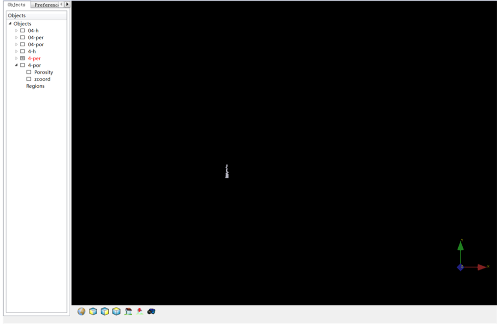
Figures 1(a)-(c) show the overview plot of the data (i.e., see original data source at Burbank Oil Fiel in Oklahoma, flow unit 5, 79 wells), and as it can be seen, under the same coordinate system, the porosity and thickness data is consistent with the well locations, indicating that they are profile of all well data, while permeability data is clustered around one well, suggesting that the permeability data may come from only one or two wells. The permeability data file only offers depth data without any X or Y coordinate which makes it one dimension data. This is a typical case shows that geostatistic data may have different scales and this usually cause difficulty in geoscience work.
3. Reservoir Data Distribution
The flow unit data contains thickness data, porosity data and permeability data
 (a)
(a)
 (b)
(b)
 (c)
(c)
Figure 1. (a) Thickness data overview of the oil field (ft); (b) Porosity data overview of the oil field; (c) Permeability data overview of the oil field (mD).
(in log form) at different X and Y coordinates. At the first step of the project, the data distribution should be viewed. Figure 2 shows the histograms of the data with bin number 8 and 12 respectively. It could be observed that as the bin number increases, the frequency of each bin decreases and this is caused by the reduction of the bin length. For example, as in Figure 2(a), it is shown that when the bin number is 8 and the frequency of the thickness that lay between 1.375 ft and 2.750 ft is 0.2. In Figure 2(b), the data is divided into 12 bins, and the frequency of the thickness that lay between 0.917 ft and 1.833 ft is zero, while the frequency of the thickness that lay between 1.833 ft and 2.750 ft is 0.2, which means all of the thickness points that lay between 1.375 ft and 2.750 ft in Figure 2(a) actually lay between 1.833 ft and 2.750 ft, and this is why the larger number of the bins, the more information the histogram could provide. Similar conclusions could be drawn from Figure 2(c) and Figure 2(d) for the porosity data and Figure 2(e) and Figure 2(f) for the log-transformed permeability data.
From the above graphs, the distributions of thickness, porosity and permeability can be observed. The coefficient of variance can be calculated as [10]

Thus, the coefficient of variance for thickness, porosity and log permeability is

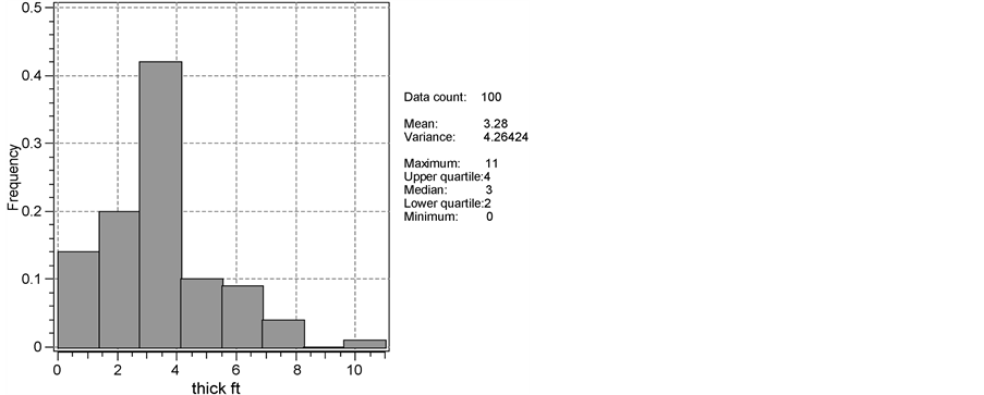 (a) Thickness histogram with bin 8 (b) Thickness histogram with bin 12
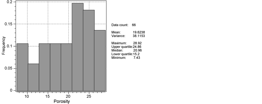 (c) Porosity histogram with bin 8 (d) Porosity histogram with bin 12
 (e) Log-permeability histogram with bin 8 (f) Log-permeability histogram with bin 12
Figure 2. The histograms of the data with bin number 8 and 12 respectively.
0.6296, 0.3146 and 0.8238 respectively. As coefficient of variance provides a relative spread of a sample and high coefficient of variance reflects the existence of extreme values. All these three are low, suggesting that there are no unacceptable outliners.
However, it is difficult to determine the exact distribution of each variable simply based on eyes judgments. Especially the distribution may look differently when different bin number is chosen. Thus, it is necessary to draw the Q-Q plots [11] to help check the distribution of the data. The samples are compared to theoretical normal distribution. If it is identical to normal distribution, a 45˚ line (red line in the graphs below) should be followed.
Figures 3(a)-(c) shows the Q-Q plot of the distribution of the variables, and from the Q-Q normal plot (a), it is very clear that there are many replicate integer numbers for thickness data and the normal distribution may not suit well

 (a) Normal QQ plot for Thickness (b) Normal QQ plot for Porosity
 (c) Normal QQ plot for Log-permeability
Figure 3. The Q-Q plot of the distribution of the variables.
for thickness data. However, for Q-Q normal plot (b), it could be observed that the data points fit well for the 45˚ line, except when the theoretical quantile is larger than 1, the fitting becomes poor and this is common when a realistic sample fits a standard normal distribution and this is the tail effect which could be tread as the outliner effect. Thus, for the porosity, except those extreme points at the two ends, the normal distribution seems well for porosity. For the permeability, since the data is log transformed and the normal distribution fits well, it indicates that the original permeability data fits well for the log-normal transformation. Thus, from the Q-Q normal plots, the distribution of the data can be known. Meanwhile, it could be used as an indication for Kriging estimation methods for later use. The thickness data, as is shown, has many replicate integer numbers and this indicates an obvious property of discrete. In this way, the multi Gaussian transformation method, which could transform the data to continuous normal form, is worthy trying. While the permeability data seems to be clustered together, which is described previously in Figure 1(c), so to estimate the overall view of permeability, Cokriging estimation based on the relationship of porosity and permeability could be applied. Also, permeability seems to follow a log normal distribution and the log transformation in nonlinear Kriging estimate method is under consideration.
After the distribution for the variables are analyzed, the relationship between variables should also be checked. Figure 4 shows the scatter plot between porosity and log permeability with its best fit line. As is shown in the graph, except for a few outlier points in the graph, the points are symmetrically scattered around the best fit line without any special trend or gathering. The correlation coefficient is 0.9425. Since it is known that the upper limit of correlation coefficient is 1, indicating a perfect positive relation of two variables, 0.9425 in this case shows that the relationship between porosity and log permeability is expectedly excellent positive linear. The regression line is

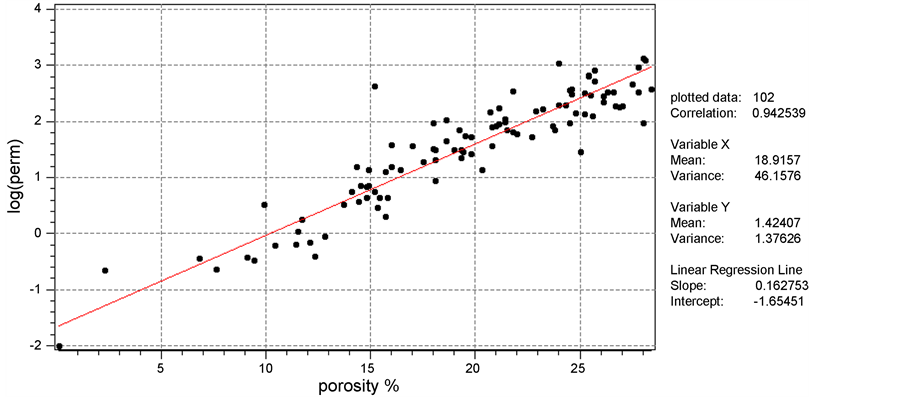
Figure 4. Relationship between porosity and log permeability.
The slope of the above equation equals , where
  is the
covariance between  and
and , and
, and  is the variance of
 .
.
4. Spatial Relationships
Variogram is used as a technique to describe the spatial relationships for geoscience data. Traditionally, there are four commonly-used basic variogram-with- still models, which is briefly shown as follows.
Nugget-Effect Model

 is the variogram at lag distance
  and
and  is the covariance at lag distance
 . If
. If ,
,  and if
 ,
,  is the still value.
Spherical Model


where  is the still value and a is the range.
Exponential Model


Gaussian Model


To make sure the pair of data is sufficient in a variogram, lag numbers, tolerance and lag separation should be carefully selected. At the beginning, the course example of thickness variograms for flow unit 5 is followed. Figure 5 shows the software set for variogram of thickness. As discussed in the class, for the number of Lags, 12 - 20 will be fine, so 12 is used. Lag Separation is the point separation in the variogram profile/graph, which is discussed as lag distance in textbook and it is half of the maximum possible distance within a region of interest, based on the rule of thumb. 1200 ft is used in this case. Tolerance respect to distance as well as direction of 10% - 50% of the separation will be fine, but mainly depends on data set. Thus, 500 ft is used for tolerance of distance and 10˚ is used for tolerance of direction. To check whether the anisotropy effect exists, we check every ten degree azimuth angle in 180˚, as based on the assumption of symmetric, the variogram will provide the same estimate by adding 180˚ to the given direction.
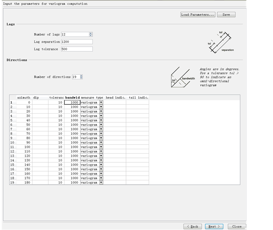
Figure 5. Software set for variograms of thickness.
The overall results for variograms of all the 19 directions could be shown in the software, then the next step is to model these variograms individually based on the four basic still models in the textbook, including Nuggget-effect, Spherical, Exponential and Gaussian, and usually Spherical model and Exponential model are used.
Also, the above obtained vairograms show different spatial continuity in different directions. Noticed that it is needed to check the anisotropic effect, the basic requirements for anisotropic models should also be applied. First, the parameters used for the variograms should be as low as possible. Second, the condition of positive definiteness should be satisfied. Third, it is assumed that directions of maximum and minimum continuity are perpendicular to each other.
Between the two basic anisotropic models, Geometric model and Zonal model, it should be realized that both these two models indicates that the structures of all variograms at different direction should be the same, the difference is that the Geometric model has similar shape and still value with different ranges, while Zonal model has different still values as well as different ranges. Thus, after simply check Geometric model is not suitable in this case because of the same still value.
The summary of model, range and still values at different directions are showed in the Table 1. Noticed that there is no Nugget-effect in all variogram structures, the consideration is as follows. First, it is very difficult to judge whether there is sufficient information for the spatial relationship as a pure nugget-effect is a sign for no quantitative information. Second, one requirement for nugget-effect model is that the shortest distance of sample pairs is larger than the range of the variogram, but after observation, there is no such sign. Third, as is mentioned, different values of nugget still show the extent of lacking information, however, it is difficult to judge the extent at different directions. For example, if after modeling, direction 10˚ may have nugget-effect still while direction 20˚ may have no nugget effect, however, is that correct to say that direction 10˚ lacks more spatial information than direction 20˚? This is obviously questionable if no other information is known. Thus, to make it more consistent and simple, one assumption in this case is that there is no nugget effect in all the variogram structures.
From the summary table, a half of a rose diagram [12] is drawn in Figure 6. Notice that the other half is just symmetric, because the variogram will provide same estimate by adding 180˚ to the given direction. Based on the table and rose diagram, it can be assumed that 0˚ and 180˚ represent the direction of the maximum continuity and 90˚ and 360˚ represent the direction of the minimum continuity.

Table 1. Variogram summary of thickness.
Similar process is done to porosity and log permeability as well and the results are shown as follows. Figure 7 shows the software set for variograms of porosity. Since as previously described, the porosity and thickness come from the same well source, which means that the location cluster behavior of the thickness and porosity are the same, the software se is same as thickness. Table 2 shows the overall results for porosity. Different to the results of thickness, the results of porosity has larger still values, while the Geometric model is, to some extent, applicable in for porosity variograms, since the still value is somewhat useful to all the plots.

Figure 6. Half of the rose diagram of lag distance in different directions of thickness data.
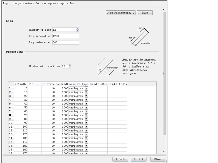
Figure 7. Software set for variograms of porosity.
As is shown in Figure 8, which is the half of rose diagram for porosity, the continuity behaviors for thickness and porosity are quite opposite, where the maximum continuity direction is 110˚ and 290˚ and minimum direction is 20˚ and 200˚. This is possible as porosity and thickness may not have strong relations. However, it is proved that porosity and permeability have strong linear relations, so the continuity of these two variables should be consistent.
Table 2. Variogram summary of porosity.

Figure 8. Half of the rose diagram of lag distance in different directions.
5. Kriging Estimation
After the variograms are modeled, the next step is to build up the grid estimation map based on the sample data. The aim of Kriging estimation is to utilize the models before to estimate values at unsampled locations with minimized variance condition. First, the data is loaded with grids divided. Figure 9 shows part of the original thickness data and the software set for the grid system built for them.
Figure 10 gives the software set for simple Kriging method for thickness grid. This means the software will use simple Kriging method to add a map of thickness for whole grid system under “4 h-grid” bar, conditioned on the thickness
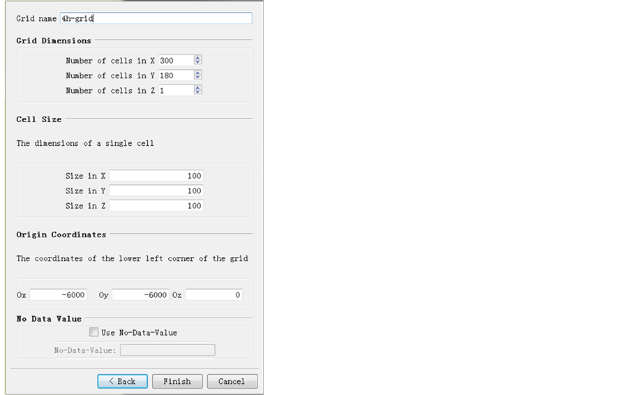
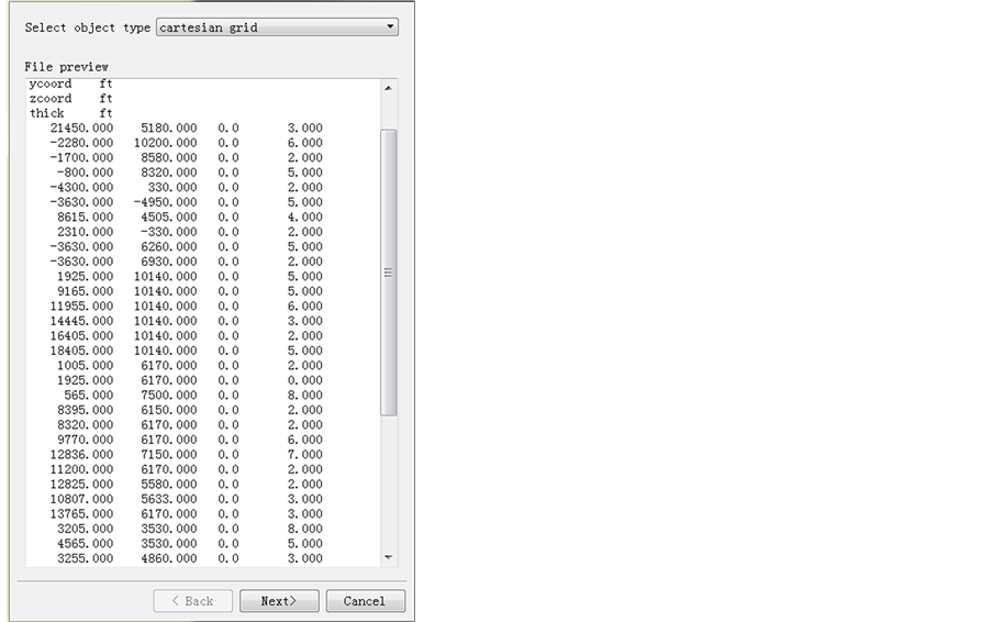
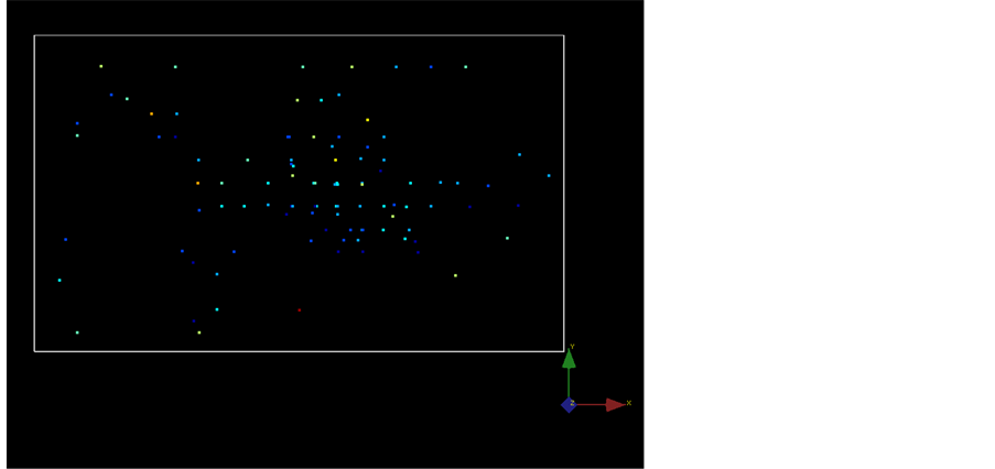
Figure 9. Software set for grid system for thickness data.
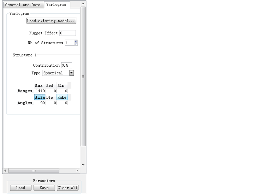
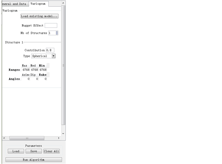

Figure 10. Software set for simple Kriging estimation for thickness data.
values in the “4 h-point” point set data. The size of the searching neighborhood is determined by the maximum range of the variograms, which could be recalled in the previous section. The searching neighborhood is set in “search ellipsoid” with searching radius of 10,000 ft, requiring a minimum of 2 data points to be found within 10,000 ft of each grid point and using no more than 12 nearest neighboring points in the estimation for each grid point.
The “variogram” tab is filled with the information on the variogram modeling of thickness which is developed before. Both range and direction of minimum continuity and maximum continuity are tried at first. The “raw” sill is set at 0.8 instead of 1.0 is to show that the raw data is applied for Kriging estimation and the structure of variogram is not exactly matched for the raw data. However, this makes no difference of 0.8 - 1.0 after carefully checking, excepting that the magnitude of the estimated Kriging variance at each grid is changed.
After simple Kriging is applied, the “Simple Kriging (SK)” bar is then changed to “Ordinary Kringing (OK)”bar, which is as shown.
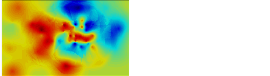
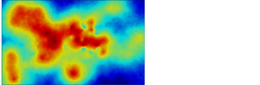
Figures 11-13 give the comparative result of simple Kriging with maximum range, a medium range of 3600, and minimum range respectively. As it can be seen, the less the range, more isolated points are shown in the map.
As it can be seen, the less the range, more isolated points are shown in the map and this is effect especially significant in the variance map. All the map of variance show a contour of variance with bull’s eyes, which indicates no spatial

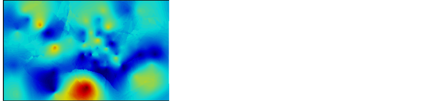
Figure 11. Simple Kriging map and variance map for thickness data (range = 6768).


Figure 12. Simple Kriging map and variance map for thickness data (range = 3600).


Figure 13. Simple Kriging map and variance map for thickness data (range = 1440).
relationship of error values, and the less the range, the bull’s-eyes effect is more obvious. This phenomenon is easy to understand, according to the definition, the grids out of the range have no spatial relationship. Thus, the less the range is set, the more isolated points in the variance map which is only at the sample location would be. It is known that the most idea case is error estimates should show no spatial correlation as values should be independent of spatial location. The range should be chosen consistent with the minimum range, since the minimum continuity direction is the principal direction and maximum continuity direction is the minor direction according to the textbook. However, since the sample data is not that sufficient, the small range cannot be chosen because the spatial relation is too ideal, which reduced the chance to know the information of other grids based on the known data. Thus, in all case of estimation below, all of the maps are built based on the maximum range of variogram. According to the textbook, the assumption that error variance is independent of surrounding samples and, in turn, of the estimated value, is called assumption of homoscedasticity. This is a typical case where the assumption of homoscedasticity is not satisfied in field data and is rarely required by the user.
Figure 14 gives the comparative result of simple Kriging and ordinary Kriging method for thickness data. Figure 15 shows the comparative variance result for each data.
Overall, the ordinary Kriging shows similar result as simple Kriging. The map has a smooth appearance with both Kriging methods. The spatial good continuity from north to south could be observed which is corresponded to the principal direction. The east to west trend which corresponds to the minor direction is less observed. The estimation variance is small in grid blocks close to the conditioning data, and it becomes larger in areas far from the data points. The variance maps of two methods has some difference, where the ordinary variance map for seems to be smoother. This is because of the ordinary method, the assumption of first-order stationary may not be strictly valid, where the local mean is dependent on the local location. This leads the estimates is relied on the neighboring girds, which produces a local average effect, making the variance seems to be smoother.
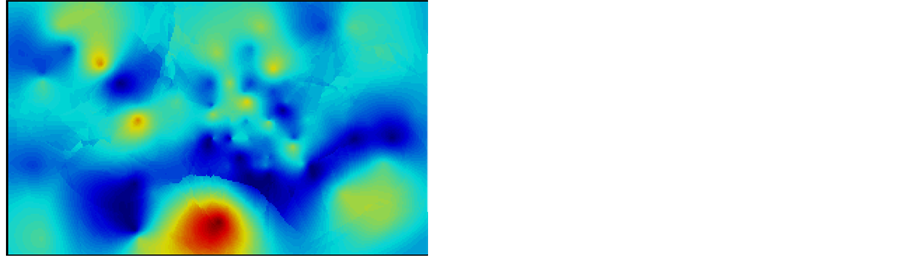
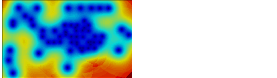
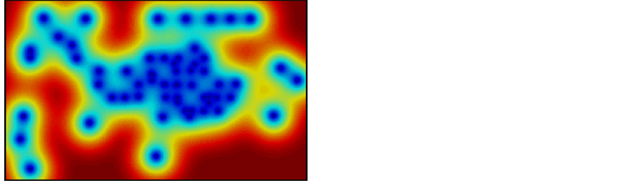
Since the porosity sample data come from the same locations, the similar process is done to porosity data as Figure 16, and the result is show in Figure 17 and Figure 18.
After observation, the difference of the results for simple Kriging method and ordinary Kriging method for porosity data seem to be obvious at the area without any data points. This is acceptable because the simple Kringing estimate of these unsampled areas relies more on the global mean, which is 19.62, while for the ordinary Kriging method, the estimate relies more on the surrounding grid

 (a) Simple Kriging map for thickness data (b) Ordinary Kriging map for thickness data
Figure 14. Kriging map for thickness data.


 (a) Simple Kriging variance map for thickness data (b) Ordinary Kriging variance map for thickness data
Figure 15. Kriging variance map for thickness data.
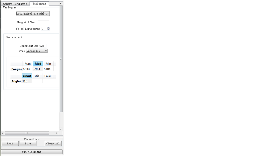
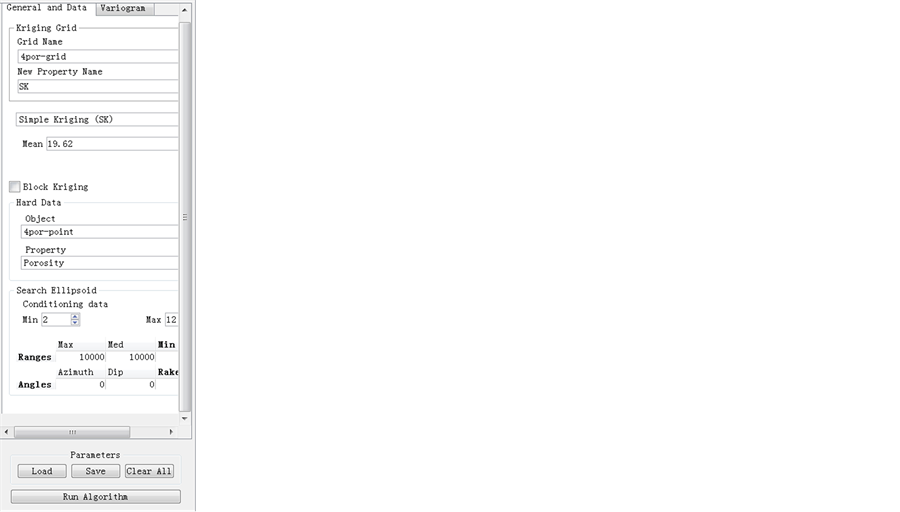
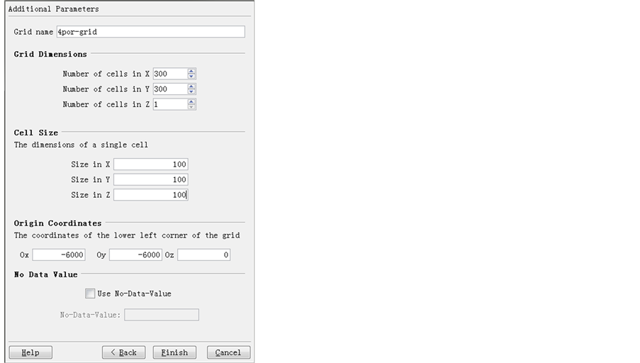
Figure 16. Software set for simple Kriging estimation for thickness data.

 (a) Simple Kriging map for porosity data (b) Ordinary Kriging map for porosity data
Figure 17. Kriging map for porosity data.
 (a) Simple Kriging variance map for porosity data (b) Ordinary Kriging variance map for porosity data
Figure 18. Kriging variance map for porosity data.
values, which vary a lot.
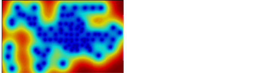
Finally, it is time to deal with the permeability data. As discussed before, permeability data is first transformed in log form. In this case, simple Kriging method, ordinary Kriging method and cokriging method are used to estimate the permeability data grid which is different from the previous grid system. At first, it is supposed to use cokriging method to estimate the whole grid system of permeability based on the linear relationship of porosity and permeability, which is checked before. However, this idea could not be realized based on the data offered for three reasons.
First, the permeability file is a one dimension data and only has depth data without any X and Y coordinate, which is shown in Figure 19. This means the searching ellipsoid should be very large to cover sufficient data points. However, Second, only the cross variogram for permeability data and porosity data can be get in the permeability data file, it is not able to get the cross variogram for the porosity data file and permeability data file. Even the minimum conditioning data is set to be only one, and the searching area covers over all the area of the grid system, there are still some unsampled location with empty surrounding grids. Thus, only the estimation for the grid system of permeability is realized.
Another way to estimate overall permeability is to use the linear relationship to estimate permeability at the all sample point of porosity. According to the definition, the equation is  and the mean of permeability will be
  with variance
 . However, this will give the exact same map as porosity, since all the points are calculated from the equation and there is no additional spatial information provided to estimate permeability.
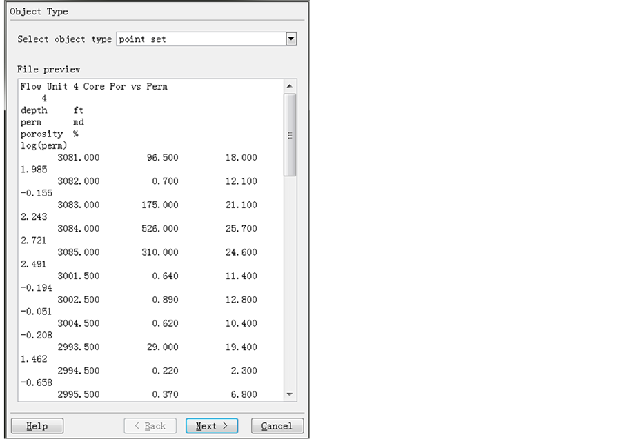
Figure 19. Data points view for porosity and log permeability.
6. Simulation
The final step is to do a simulation with attempt to find the difference between simulation method and estimation method. Sequential Gaussian Simulation is used in this case, which assumes that the normalized local error variance follows a standard normal distribution. The software set for thickness data for the method is shown in Figure 20. The seed is used to generate random numbers. Since simulation will use random generator, the software will use seed as reference, different seed will give different random numbers which will lead different results. The student ID is used as seed in this case.
The result for one simulation realization with seed 359,357 for thickness data is shown as Figure 21. To be more informative, another realization is also done with seed 200.
Obviously, from the above two graphs, simulation with different seed numbers will result different map. Simulator will generate different random numbers
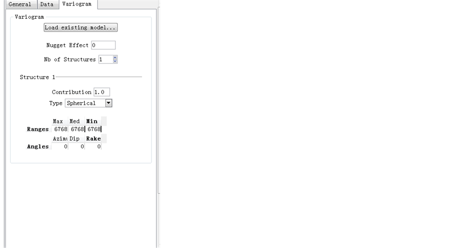
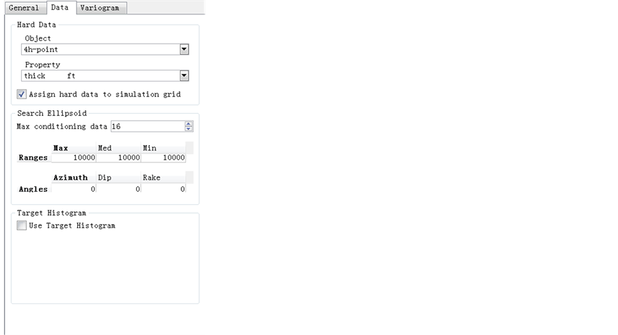
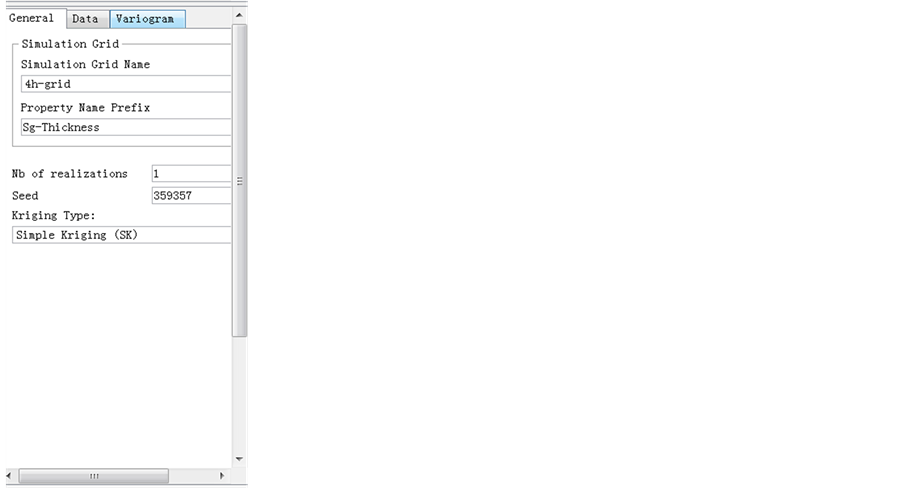
Figure 20. Software set for thickness simulation.

 (a) Simulation realization with seed 359,357 for thickness (b) Simulation realization with seed 200 for thickness
Figure 21. Simulation realization with different random seed for thickness.
each time. They have equal probability, but since each grid is with different value, the overall map the looks quite varied.
Then the simulation results are compared with Kriging estimation, which are shown in Figure 22.
As is discussed, the estimation is to minimize error variance, while the simulation technique is to simulate reality. The sequential Gaussian simulation is a conditional simulation method, which provides the local variability by creating alternate, equiprobable images follows normal distribution instead of defining and estimate. The uncertainty is then characterized by multiple possibilities that exhibit local variance. Since it assumes a continuous normal distribution, as it can be observed, although grid values are different in two maps, the change in the simulation result is not as sharper as in the estimation method. The sequential Gaussian simulation gives a smoother result.
The similar results for porosity are in Figure 23 and Figure 24. Compared to the result simple Kriging method result Figure 22(a) and ordinary Kriging method result Figure 22(b), the same conclusion as above will be drawn.
7. Conclusion
In the early stage of geostatistics, which is before the production of the reservoir with the limited amount of information, the reservoir description has more


 (a) Simple Kriging map for thickness data (b) Ordinary Kriging map for thickness data
Figure 22. Kriging maps for thickness data.

 (a) Simulation realization with seed 359,357 for porosity (b) Simulation realization with seed 200 for porosity
Figure 23. Simulation realization with different random seed for porosity.

 (a) Simple Kriging map for porosity data (b) Ordinary Kriging map for porosity data
Figure 24. Kriging maps for porosity data.
uncertainty. The reservoir characterization is realizable in this stage by using computers to solve the upscale and heterogeneity problem. The whole map of the properties of the reservoir could be drawn based on the discrete local information of the reservoir. However, the accuracy of these descriptions is very hard to be determined, as the real situation in the reservoir formation is unknown. Different engineers may have different understanding of the data as the analysis process cannot avoid subjective judgments. Thus, the reservoir characterization should be updated in time once new information is available.
Grant Numbers
2016ZX05060026 (Thirteen-Five National Science and Technology Major Projects: Study on Shale Gas Fracturing and Gas Production Regularity in Wufeng Formation and Longmaxi Formation in Fuling Area), 2016ZX05025001 (Thirteen-Five National Science and Technology Major Projects: Study on the Fine Representation of Residual Oil of Offshore Sandstone Heavy Oil Reservoir Based on the Nonlinear Fluid Flow), 2016ZX05027004 (Thirteen-Five National Science and Technology Major Projects: Study on the Key Techniques for Effective Development of Large-scale Gas Field in Thick Heterogeneity of East China Sea).
Cite this paper
Zhang, M.L., Zhang, Y.Z. and Yu, G.M. (2017) Applied Geostatisitcs Analysis for Reservoir Characterization Based on the SGeMS (Stanford Geostatistical Modeling Software). Open Journal of Yangtze Gas and Oil, 2, 45-66. https://doi.org/10.4236/ojogas.2017.21004
References
- 1. Kelkar, M. and Perez, G. (2002) Applied Geostatistics for Reservoir Characterization. Society of Petroleum Engineers, Richardson, Texas, 30-50.
- 2. Webber, K. J. and Van Geuns, L.C. (1990) Framework for Constructing Clastic Reservoir Simulation Models. Journal of Petroleum Technology, 42, 1-248.
- 3. Lucia, F.J. (1983) Petrophysical Parameters Estimated from Visual Descriptions of Carbonate Rocks: A Field Classification of Carbonate Pore Space. Journal of Petroleum Technology, 35, 629-637.
https://doi.org/10.2118/10073-PA - 4. Chilès, J.P., Aug, C., Guillen, A. and Lees, T. (2004) Modelling the Geometry of Geological Units and Its Uncertainty in 3D from Structural Data: The Potential-Field Method. Proceedings of International Symposium on Orebody Modelling and Strategic Mine Planning, Perth, 24 p.
- 5. Myers, D.E. (1988) Vector conditional simulation. In: Armstrong, M., Ed., Geostatistics, Kluwer, Dordrecht, 283-292.
- 6. Davis, M.W. (1987) Production of Conditional Simulations via the LU Triangular Decomposition of the Covariance Matrix. Mathematical Geology, 19, 91-98.
- 7. Verly, G.W. (1993) Sequential Gaussian Cosimulation: A Simulation Method Integrating Several Types of Information. In: Verly, G.W., Ed., Sequential Gaussian Cosimulation: A Simulation Method Integrating Several Types of Information. Geostatistics Troia’92, Springer, Netherlands, 543-554.
https://doi.org/10.1007/978-94-011-1739-5_42 - 8. Boucher, A. and Dimitrakopoulos, R. (2009) Block Simulation of Multiple Correlated Variables. Mathematical Geosciences, 41, 215-237.
https://doi.org/10.1007/s11004-008-9178-0 - 9. Desbarats, A.J. and Dimitrakopoulos, R. (2000) Geostatistical Simulation of Regionalized Pore-Size Distributions Using Min/Max Autocorrelation Factors. Mathematical Geology, 32, 919-942.
https://doi.org/10.1023/A:1007570402430 - 10. Davis, J.C. (1986) Statistics and Data Analysis in Geology. John Wiley & Sons, New York.
- 11. Issaks, E.K. (1989) Applied Geostatistics. Oxford University Press, New York.
- 12. Davis, B.M. (1987) Uses and Abuses of Cross-Validation in Geostatistics. Mathematical Geology, 19, 241-248.
https://doi.org/10.1007/BF00897749