International Journal of Geosciences
Vol.5 No.9(2014), Article
ID:48940,18
pages
DOI:10.4236/ijg.2014.59080
Influence of the Freshwater Discharge on the Hydrodynamics of Patos Lagoon, Brazil
Gustavo Pessoa de Barros1, Wiliam Correa Marques2, Eduardo de Paula Kirinus1
1Institute of Oceanography, Federal University of Rio Grande, Rio Grande, Brazil
2Institute of Mathematics, Statistics and Physics, Federal University of Rio Grande, Rio Grande, Brazil
Email: oc.gustavobarros@gmail.com
Copyright © 2014 by authors and Scientific Research Publishing Inc.
This work is licensed under the Creative Commons Attribution International License (CC BY).
http://creativecommons.org/licenses/by/4.0/


Received 14 May 2014; revised 12 June 2014; accepted 8 July 2014
ABSTRACT
Patos Lagoon is a very dynamic environment presenting hydrodynamic fluctuations from synoptic to decadal timescales. Thus, understanding the processes that determine the long term variability is fundamental for the correct coastal planning and management of this region. The main objective of this study is to understand how the freshwater discharge of the main tributaries controls the estuarine hydrodynamics of the Patos Lagoon, when considering long term timescales. Two numerical simulations were carried out using the TELEMAC3D numerical model, the former using freshwater discharge from 1940 to 1973 year (simulation A), and the second simulation using data between 1974 and 2006 year (simulation B). These two periods were selected because before (after) 1973 year, the annual mean freshwater discharge was lower (higher) than the mean value for the whole period (1080 m3/s). The navigational channel discharge, water level, salinity and current velocity differences between both simulations were analyzed. Ebb conditions prevailed over flood conditions for both simulations, but simulation B presented a higher volume of freshwater exported through the coastal zone. Water level differences demonstrated higher values (0.08 meters) close to the Guaiba River, which is the main tributary of the study region, and lower values were observed near to the Patos Lagoon mouth (0 meters). The most significant differences in the mean bottom and surface salinity were observed in the central zone of the estuary and at the Barra Breakwaters. Simulation A presented higher saline intrusion due to lower freshwater discharge, while simulation B showed an increase in the coastal plume intensity, caused by the higher freshwater discharge. The hydrodynamical simulations demonstrated with precision that the freshwater discharge intensity determine the vertical stratification of the estuary.
Keywords:Estuarine Hydrodynamics, Freshwater Discharge, Hydrodynamical Modeling

1. Introduction
Estuarine circulation is normally controlled by the wind action, tides and freshwater discharge [1] . In micro-tide regions, over synoptic time scales, the wind effect is the most important forcing controlling the exchange processes between the estuarine and coastal regions [2] . On the other hand, at longer time scales (months, years and longer), the freshwater discharge becomes extremely important controlling the estuarine hydrodynamics. The Patos Lagoon estuary demonstrates the pattern described above.
At long time scales, South America is influenced by the El Niño Southern Oscillation phenomenon (ENSO) [3] [4] . The ENSO phenomenon is a natural climate fluctuation with the most intense interannual scale. This phenomenon can be described as a low frequency irregular oscillation between a warm (El Niño) and cold (La Niña) state [5] . The South of Brazil shows precipitation anomalies caused by the occurrence of ENSO events. During El Niño years the spring tends to be weather and during La Niña years droughts anomalies occur [6] [7] .
The freshwater discharge fluctuations caused by changes in precipitation associated with cold front passages and ENSO events are very important on the hydrodynamical control of Patos Lagoon. These fluctuations can affect a large number of processes that are social, ecological and economically important (e.g., influence on the reproduction and survival of fauna and flora, increase/decrease the quantity of flooded areas, affect the productivity of rice and corn production, etc.).
In the past years, increases in water levels at Patos Lagoon resulted in the dislodgement of a vast number of families that inhabit the region’s islands. These events are responsible for eroding the lagoon and island’s margins, causing land losses, altering ecosystems and affecting socio-economic activities in the region [8] . The intensity of freshwater discharge also controls the formation of the Patos Lagoon’s coastal plume which is very important on the sediment transport and estuarine stratification [9] .
During El Niño years, the increase of freshwater discharge intensifies ebb conditions, which prevents the entrance of shrimp larvae and other economically important species on the lagoon, resulting in severe socio-economic problems for the local fishermen [10] . During La Niña years, the salt water that enters the estuary can reach distances of 180 km from the Patos Lagoon’s mouth, reducing the productivity of rice plantations along the lagoon that are responsible for one quarter of the state’s total rice production [11] .
According to Timmermann et al. [5] , climate changes on the tropical Pacific region can increase the occurrence of ENSO events and result in a higher interannual variability, which would cause extreme variations in climate conditions each year. These climate changes can be associated with the temperature raise, which would probably reduce the intensity of trade winds, cause the tropical regions to heat faster than the poles, increase the temperature gradients along the thermocline and reduce the thermocline thickness [12] .
It’s possible to estimate that the seasonal and interannual pattern of the Patos Lagoon’s freshwater discharge will change significantly due to changes in precipitation caused by climatic global changes. In this way, it’s essential to understand how the discharge controls the estuarine circulation, exchange processes between estuary and ocean, salinity distribution and water level variations at longer time scales, making it possible to estimate how these changes will affect the region’s hydrodynamics, and consequently, fisheries, agriculture and economy. The main objective of this paper is to understand how the freshwater discharge controls the estuarine hydrodynamics in long time scales.
2. Description of the Study Area
Patos Lagoon is located in the southernmost part of Brazil, between latitudes 30˚S - 32˚S and longitudes 50˚W - 52˚W (Figure 1) and it’s considered the largest choked coastal lagoon in the world [13] . Patos Lagoon has a surface area of 10,360 km2, is 250 km long and 40 km wide, draining a watershed of approximately 201,626 km2. The estuarine region covers about 10% of the total area [14] . The freshwater reaches the adjacent coastal zone through the Barra Breakwaters.
The three main contributing rivers are Taquari and Jacuí, which flows through the Guaíba River in the northern region of the lagoon, and Camaquã River, which flows into the central region of the lagoon. The tidal oscillation (0.4 m) is of secondary importance at the estuarine circulation [10] .
On interannual time scales, the freshwater discharge is responsible for 50% of the water level fluctuations at the estuary and 80% at the lagoonar region [15] . Barros and Marques [15] verified the occurrence of interannual events (reaching from 1.5 to 6 years) associated with ENSO controlling the freshwater discharge and water levels at Patos Lagoon.
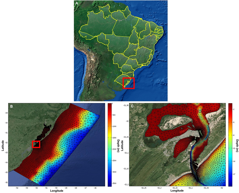
Figure 1. Location of the study area in the South of Brazil (A), study area and grid used in the numerical simulations (B) and estuarine region zoomed (C). Red boxes indicate the area zoomed at the images.
3. Methodology
3.1. Numerical Model
The numerical model used to investigate the influence of the freshwater discharge on Patos Lagoon’s hydrodynamics was the TELEMAC system, developed by the Laboratoire National d’Hydraulique of the Company Electricité de France (EDF). The numerical model is based on the finite element methods [16] and presents a modular structure, being able to perform two and three dimensional simulations, offering modules for waves, hydrodynamic, sediment transport and water quality studies in rivers, estuaries, coastal and oceanic regions.
The modules used in the present study were: MATISSE, TELEMAC3D and POSTEL3D. The first one allows the generation of the bathimetric grid and initial and boundary conditions for the domain. The second module solves the Navier-Stokes equations for free surface flows accepting the hypothesis of hydrostatic equilibrium, assuming the free surface flow with boundary conditions generated from wind stress. The last one is a postprocessing module, which is responsible for extracting vertical profiles from the bathimetric grid, allowing the analysis of the water column.
The numerical model also considers the free surface evolution as a function of time, using the advection-diffusion equations to calculate the transport of the tracers concentrations (e.g., salinity, temperature or sediments in suspension). These average approximations have been proved to be suitable for applications in shallow water, in regions where the vertical velocities are smaller than the horizontal. For a complete description of the physical, mathematical and computational development of the numerical model TELEMAC, consult Hervouet [16] .
A great number of studies have been conducted using the TELEMAC model in the Southern region of Brazil. These studies described coastal plume dynamics, estuarine circulation, sediment dispersion and the energy potential of currents [17] -[20] . The calibration and validation of the TELEMAC3D for the study area has already been performed by Marques et al. [17] -[19] . In the present study, the same parameters used by these authors were applied, therefore, validation and calibration tests will not be demonstrated here.
3.2. Bathimetric Grid
The bathimetric grid is composed by 19.211 triangular elements and 10.366 nodes, where the equations are processed by the numerical model. The grid is defined between latitudes 28˚S and 36˚S and between longitudes 46˚W and 54˚W. Using these coordinates, the Patos Lagoon region is totally covered, as well as the adjacent coastal zone until approximately 3700 meters depth. The average depth in the lagoonar region is approximately 10 meters and at the estuarine region the maximum depth is 18 meters in the navigation channel (Figure 1(C)). Since the aim of this study is to investigate the estuarine circulation, the non-structured bathimetric grid is more refined in this area, which presents a larger concentration of elements and nodes than the coastal area (Figure 1(C)).
3.3. Initial and Boundary Conditions
In order to carry out the numerical simulations, TELEMAC3D requires the prescription of salinity, temperature, water level and velocity fields as initial conditions. Salinity and temperature fields are obtained from the OCCAM Project (Ocean Circulation and Climate Advanced Modeling Project—http://www.soc.soton.ac.uk/), and prescribed three-dimensionally over the entire domain.
The tides are prescribed for the eastern oceanic boundary at each nodal point using the amplitude and phase of each of the five principal tidal components for the area: K1, M2, N2, O1 and S2 [21] . These components are obtained from the Grenoble Model (FES95.2, Finite Element Solution—v.95.2).
The surface boundary of the model is forced with space and time variable winds from reanalysis (National Oceanic & Atmospheric Administration—NOAA, www.cdc.noaa.gov/cdc/reanalysis), which are prescribed at each nodal point of the mesh. These data are obtained with temporal resolution of 6 hours. The freshwater discharge from the main contributing rivers, Taquari, Jacuí and Camaquã Rivers, is used as continental liquid boundary. The data is collected by the Brazilian National Water Agency (ANA—www.ana.gov.br).
3.4. Data and Parameters
All the data used on the numerical simulations were transformed in long term means. Salinity, water levels, temperature and current speed and direction data covers the period from 1990 to 2004 year (OCCAM). Air temperature and wind speed and direction data range from 1948 to 2010 year (NOAA). Freshwater discharge data covers the period between 1940 and 2006 year (ANA).
The parameters used in the simulations are the same used by Marques et al. [17] -[19] , and can be seen on Table1 Two simulations over 365 days of duration were performed using the same data, except for the freshwater discharge. This parameterization was applied in order to identify the influence of the freshwater discharge on the estuarine hydrodynamics.
Analyzing freshwater discharge time series from 1940 to 2006 year, Marques [22] obtained an annual mean discharge of 1080 m3/s for the main contributing rivers of the Patos Lagoon. Furthermore, this author observed that until (after) 1973 the annual mean was below (above) the average value. In the present study, these time series were applied in two different numerical simulations: the former one using the annual mean values from 1940 to 1973 year (simulation A) and the second one from 1973 to 2006 year (simulation B) (Figure 2).
4. Results and Discussion
4.1. Freshwater Discharge
The annual freshwater discharge was calculated for both simulations by summing the daily values over 365 days

Table 1 . Parameters used in the numerical simulations.
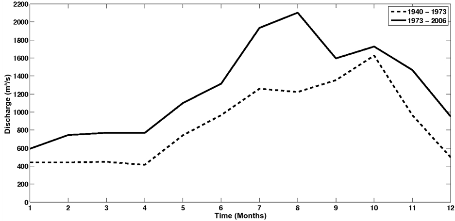
Figure 2. Climatological mean of the freshwater discharge between 1940 and 1973 (dotted line) and from 1973 to 2006 (solid line) (Adapted from Marques [22] ).
of simulation (Table 2). The annual discharge rate of the channel considers the amount of water that enters and exits into the channel, where positive (negative) values indicate flood (ebb) conditions (Figure 3). The integrated time series of the freshwater discharge defines the daily discharge for the simulated period.
Due to the higher freshwater discharge intensity in simulation B, the liquid annual discharge values were superior to simulation A. In this way, after 1973 year the liquid annual discharge increased 18.45% when compared to the period between 1940 and 1973 year. The mean daily discharge increased 0.21 × 10³ m3·s−1 after 1973 year. The mean channel discharge increased 13.71% after 1973 year. These results indicated that Patos Lagoon increased the volume of freshwater exported towards the coastal zone, which affects the intensity of the coastal plume, salinity distribution and stratification.
The integrated time series of the freshwater discharge indicates that ebb conditions prevail over flood conditions, indicating that there is more freshwater reaching the adjacent coastal region than salt water entering into the estuarine zone. It is possible observe that during flood conditions (positive values) the simulation A demonstrates higher values than simulation B, due to the lower intensity of the freshwater discharge. On the other hand, during ebb conditions (negative values) simulation B presents higher discharge intensity than simulation A.
According to Marques et al. [23] , the Patos Lagoon estuary presents a residual circulation pattern favorable to
Table 2 . Values of liquid annual discharge, mean channel discharge, mean daily discharge for simulations A and B, difference and increase percentage between A and B.
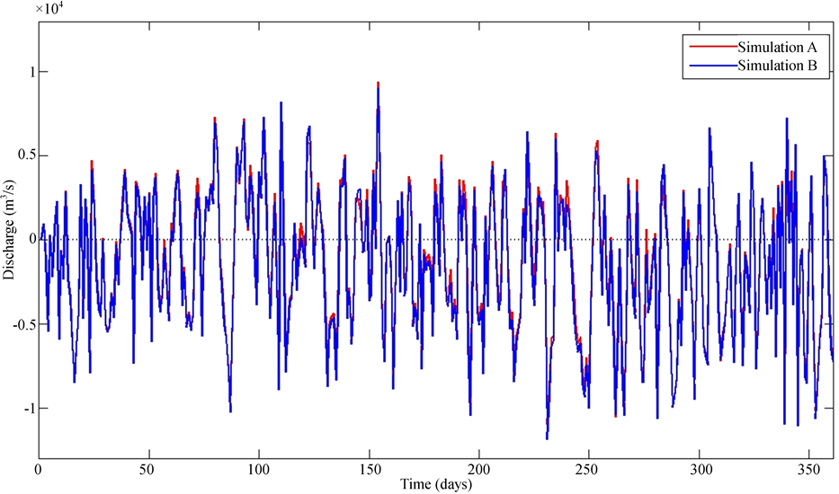
Figure 3. Integrated time series of the freshwater discharge for the 365 days simulated.
the ebb conditions independent of the freshwater discharge, while the mean stratification along the estuary is controlled by the intensity of freshwater discharge. Under normal meteorological conditions, the flooding events occur periodically during the whole year. In this sense, the effective intrusion of the oceanic waters, as well as, the vertical and horizontal stratification is directly related to the intensity of the freshwater discharge of the Patos Lagoon river tributaries [23] .
4.2. Water Level
The results indicate the influence of the freshwater discharge on the water levels of Patos Lagoon. It can be observed that the difference in the lagoonar region is superior to the observed at the estuarine region (Figure 4). This result indicates that the lagoonar region is more influenced by the freshwater discharge, due to its proximity to the main tributaries of Patos Lagoon (Jacuí, Taquari and Camaquã rivers), than the estuarine region, which is affected by the coastal processes of the adjacent ocean. According to Möller et al. [11] , meso and large scale circulation, as well as, the remote action of the wind are important physical factors controlling the estuarine circulation.
The difference between the mean water level between simulations A and B is represented in Figure 4. The difference was calculated by subtracting the mean value of A from B. The positive values indicate that the water level is directly proportional to the freshwater discharge. The maximum value of 0.08 meters is observed near to the Guaíba river, which is the main tributary of the lagoon. The difference value gradually reduces from the north part of the lagoon until it reaches the minimum value of 0 meters in the lagoon’s mouth and oceanic area.
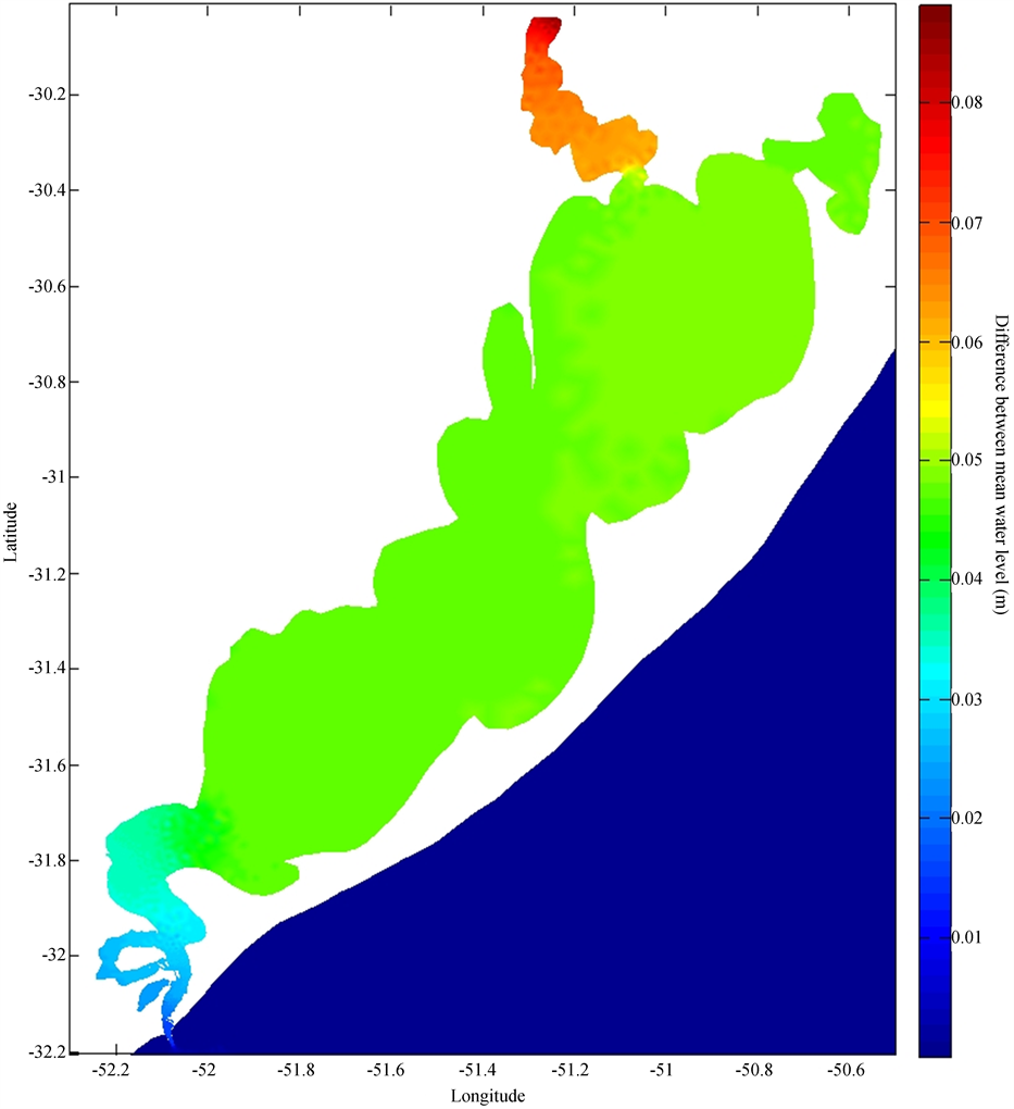
Figure 4. Mean water level difference between simulations A and B. The difference was calculated by subtracting the mean value of A from B (Difference = mean B – mean A).
The results from the numerical simulations corroborate the results obtained by Barros and Marques [15] , which determined that in long time scales, the freshwater discharge is responsible for 50% of the water level fluctuation in the estuarine region and 80% at the lagoonar portion.
The difference may seem small, but can definitely affect a large number of processes that are social, ecological and economically important (e.g., influence the reproduction and survival of fauna and flora, increase/decrease the quantity of flooded areas, affect the productivity of rice and corn production, etc.). In the past years, increases in water levels at Patos Lagoon resulted in the dislodgement of a large number of families that inhabit the region’s islands. Salinity fluctuations caused by water levels changes and wind intensity and direction are responsible for determining the composition of species, diversity and abundance of the benthic macrofauna [24] .
4.3. Surface Salinity
Analyzing the difference values between simulations A and B (Difference = mean B − mean A) is possible do identify areas with salinity variation of approximately 1.6 psu (Figure 5). The negative difference values for most of the estuarine area is expected since we are subtracting a higher salinity value (simulation A, forced with lower freshwater discharge) from a lower salinity value (simulation B, forced with higher freshwater discharge).
The salinity distribution demonstrated the same pattern observed by another authors [15] [17] [19] [23] , in which the salinity at Patos Lagoon is proportionally inverse to the freshwater discharge. The simulation B presented lower salinity values than simulation A in most of the estuarine region, except for two regions with positive difference values on the Mangueira Bay and the west region of the Marinheiros Island (areas in red). These two choked regions present an area with reduced circulation which decreases the exchange processes under conditions of higher freshwater discharge. This hydrodynamic pattern increases the saline intrusion and the residence time of the salt water causing these positive difference values.
The construction of a bridge at the connecting region between the Mangueira Bay and the lower part of the estuary resulted in the strangulation of the passage between these two areas. The reduced passage caused a significant increase in the current velocity, which resulted in intensive erosion that changed local depth from 3 meters to 14 meters [25] . The bridge also reduced the exchange rate between the estuary and the Mangueira Bay reducing the water renewal rate and increasing the residence time.
Salinity variations of 2 psu can affect dissolved inorganic nutrient cycling, which are the main source of energy for macro and microalgae placed at the bottom of the trophic chain at the Patos Lagoon ecosystem. These algae are responsible for the high organic matter productivity in this region. In salinities lower than 5 psu, nutrients

Figure 5. Mean surface salinity difference between simulations A and B at the estuarine region. The difference was calculated by subtracting the mean value of A from B (Difference = mean B – mean A).
are resuspended by flocculation and particle removal processes. In intermediate salinities (5 to 27 psu), the dominant process is the sediment remineralization, while in high salinities (higher than 27 psu) linear changes occur in nutrients concentrations, due to mixing processes of different water masses [26] .
The area that presented higher difference between mean surface salinity was the central region of the navigational channel of the Rio Grande port and its proximities. This region, besides having an elevated exchange process rate between fresh and salt water is also constantly dredged to increase the navigational channel by removing sediment.
Channel sediment removal alters the local bathimetry and morphodynamics. In addition, the combination with alongshore winds, freshwater discharge and tide amplitude control the circulation processes at the estuarine region. According to Möller and Fernandes [27] , morphological changes induced by dredging, bridges and other structures, can affect tidal waves propagation, modify vertical salinity stratification and alter salinity intrusion into the estuarine zone.
The mean freshwater exportation increased for the simulation B at the lagoon’s mouth, due to the higher discharge intensity. The increase of freshwater contribution at the adjacent coastal area also increases the intensity of the coastal plume. This higher exportation observed in simulation B may alter the behavior of the Patos Lagoon’s coastal plume, which is fundamental for the fine sediment transport in the region [19] . The spatial and temporal variability of freshwater fish species is also affected by the increased reach of the freshwater, demonstrating an inverse correlation with the salinity [28] .
4.4. Bottom Salinity
The pattern presented by the bottom salinity (Figure 6) is similar to the surface salinity, in which simulation B
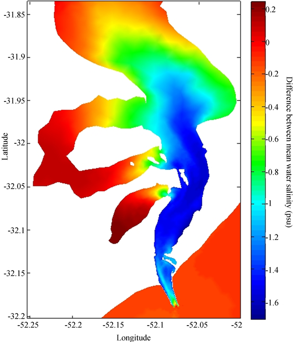
Figure 6. Mean bottom salinity difference between simulations A and B at the estuarine region. The difference was calculated by subtracting the mean value of A from B (Difference = mean B – mean A).
demonstrated lower values for almost all the estuarine region, except for the two strangled areas (highlighted in red). Simulation A demonstrated a higher saline intrusion into the estuarine zone, due to the lower freshwater discharge intensity. The saline wedge in simulation A, reaches a distance of 2 km higher than simulation B. Since salt water is denser than freshwater, this saline intrusion difference is well represented in the mean bottom salinity.
The most significant differences in the mean bottom salinity are found in the central region of the estuary and at the lagoon’s mouth channel. In these regions, simulation B presented values of 1.7 psu lower than simulation A, demonstrating the same pattern observed in the mean surface salinity. It is not possible to observe any differences in the coastal plume intensity at the bottom salinity image (Figure 6), since freshwater is less dense than salt water, occupying the surface layers of the water column.
The higher intrusion of saline water in the estuary remobilizes the sediment, which may promote a higher aport of ammonium and phosphate in the water column [29] . Thus, the increased flux of freshwater discharge in the system could result in a lower liberation of sediment nutrients, reducing drastically the concentration of dissolved inorganic nutrients for the primary producers.
Liu et al. [30] performed hydrodynamical simulations of the Tanshui estuary, Taiwan, China, using low intensity freshwater discharge. The salinity values were between 1 and 2 psu superior than the salinity values obtained in simulations with high freshwater discharge. The saline intrusion limits in low discharges were determined by the local bathimetry [30] .
The composition, density and biomass of the microalgae community at the Patos Lagoon’s estuary is directly dependent on the salinity pattern in the region [31] . Thus, this reduction observed in the mean salinity after 1973 year, may affect the macroalgae community, which is responsible for the main primary production in the study area. In shallow regions of the estuary, the highest density, chlorophyll-a and biovolume values are associated with periods of low salinity [31] .
Liu et al. [32] , determined that the reduction in freshwater discharge increases by 4, 6 and 14 km the saline intrusion at the estuaries of Hsintien, Keelung and Tahan, China, respectively. These authors found a high correlation between the freshwater discharge and the saline intrusion, in which the reach of the saline intrusion reduces exponentially with the increase of the freshwater discharge. The correlation was higher than 0.9, indicating that the numerical model can be used to estimate the saline intrusion under the influence of the freshwater discharge of the main tributaries [32] . This technique can be used to predict the salinity fluctuation at the estuarine region.
Dat et al. [33] found a correlation of 0.87 between the saline intrusion and the freshwater discharge at the Mekong river estuary, Taiwan, China. This result was used to decide whether or not to build structures to control the salinity in the Mekong and Bassac rivers, in case of climate changes and reductions on the freshwater discharge.
4.5. Vertical Salinity
Vertical profiles were extracted to evaluate the variations of the circulation pattern along the water column caused by the different freshwater discharges (Figure 7).
The areas selected for the vertical profiles were: the Patos Lagoon’s mouth (P1), the beginning of the Barra Breakwaters (P2) and a longitudinal profile along the Barra Breakwaters (P3). These areas were selected due to their importance for the estuarine hydrodynamics.
Comparing profiles for simulations A and B in P1 (Figure 8), it can be observed that the vertical salinity gradient is more accentuated in simulation B. Below 13 meters depth, both simulations present similar salinity values between 33 and 34 psu. In the first 3 meters, the salinity in simulation A is approximately 28 psu, while in simulation B some points show salinity values lower than 26 psu.
The halocline is defined as a zone of rapid salinity increase with depth [34] and is represented by the green area with salinity values between 29.1 and 30.7 psu. In simulation B, the halocline showed lower salinity values than simulation A. It is also possible to observe a variation in the halocline position. In simulation A the halocline is located between 8 and 11 meters depth. On the other hand, in simulation B the halocline sinks and reaches depths between 10 and 13 m. Abrosimova et al. [35] observed a sinking of the halocline position in the Amurskiy Liman and Sakhalin bays, Okhotsk Sea (Asia), during conditions of lower salinities caused by the increase of freshwater discharge from the Amur River.

Figure 7. Local depth at the Barra Breakwaters region and location of the vertical profiles P1, P2 and P3. The profiles begin at the circle mark and end in the square mark.
In both simulations it is possible to observe that the saltier water near the bottom moves westward, while the surface layer, which is less dense, moves eastward. This advection movement results in the increase of salinity in the first meters of the water column. The velocity vectors do not present any significant differences for simulations A and B indicating that the freshwater discharge does not affect considerably the direction and intensity of the estuary’s vertical circulation near the Patos Lagoon mouth.
In Figure 9, it is possible to observe that the salinity gradient in P2 is more accentuated than in P1, which was expected since P2 is more distant to the mouth than P1, increasing the dominance of the freshwater discharge and reducing the effect of the adjacent coastal circulation on the salinity control.
The salinity difference between simulations A and B is noticeable in both the surface and bottom layers. In simulation A, the salinity values are approximately 25 psu for the first 3 meters depth. For the simulation B, this value is reduced to 23 psu, indicating a variation of almost 2 psu in some points. Under 11 meters depth, the simulation A demonstrates salinity values higher than 28 psu, while in the simulation B these values are lower than 27 psu.
It is also possible to verify a change in the halocline position, as well as in P1. In simulation A, the halocline is located between 3 and 7 meters depth, while in simulation B the halocline sinks reaching depths between 7 and 11 m. The halocline sinking indicates that there is more freshwater reaching higher depths in the water column. In both simulations the halocline sinked at the navigational channel region, which presents higher
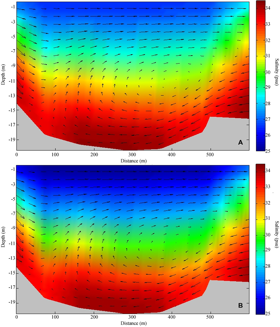
Figure 8. Mean salinity and current direction vertical profiles (P1) for simulations A and B.
depths of approximately 16 m. Chant and Wilson [36] observed that in ebb conditions, the halocline tends to follow the channel depth, sinking (raising) in regions with higher (lower) depths.
As well as in P1, the water circulation direction for P2 was east-west on the bottom and the opposite on the surface. It can be seen in both simulations the advection movement that increases salinity in the superficial layers of the water column. The circulation pattern, current intensity and direction were similar in both simulations.
Marques et al. [23] investigated the variability in exchange processes at Patos Lagoon comparing an El Niño year (with elevated freshwater discharge) with a normal meteorological condition year (with average freshwater
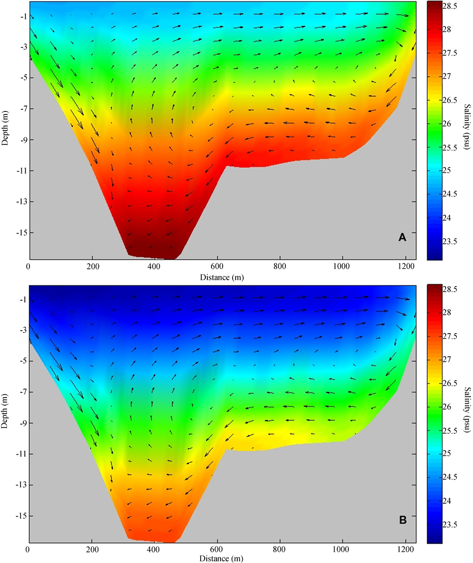
Figure 9. Mean salinity and current direction vertical profiles (P2) for simulations A and B.
discharge), using the TELEMAC3D model. The simulations demonstrated that the Patos Lagoon estuary presents a residual circulation pattern favorable to ebb conditions independently of the freshwater discharge. However, the mean vertical and horizontal stratification along the estuary is strongly dependent on the intensity of the freshwater discharge [23] . The freshwater discharge is also responsible for determining the occurrence and reaching of the saline intrusion.
The vertical profile (Figure 10) represents the longitudinal channel of the Barra Breakwaters, starting at the estuarine region and finishing at the oceanic zone (from 3000 meters and beyond). In both images (A and B) it is noticeable that the water in the first meters of the water column moves towards the ocean, demonstrating a mean ebb condition pattern. The vertical and horizontal circulation pattern is similar in both simulations, reinforcing that the freshwater discharge intensity does not affect the direction and intensity of the currents.
In the surface, there is a salinity difference of almost 2 psu between simulations A and B. Simulation B
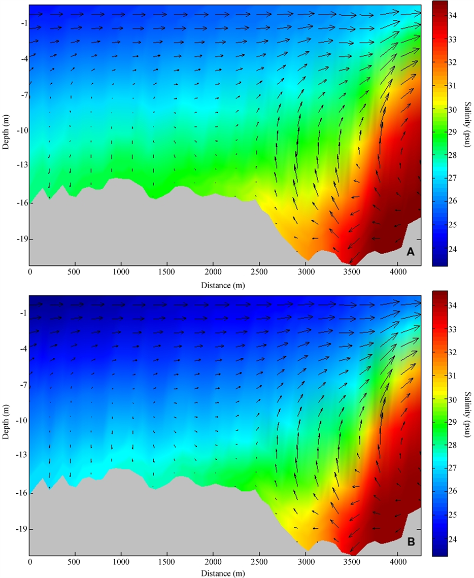
Figure 10. Mean salinity and current direction vertical profiles (P3) for simulations A and B.
presented higher homogeneity (i.e. the water column was less stratified) from the beginning of the profile up to the distance of 1600 meters length. Simulation A presents higher stratification in the same section, caused by the reduced intensity of the freshwater discharge.
Liu et al. [37] found a similar pattern at the estuary of Danshuei River, China. These authors used numerical modeling techniques to identify higher stratification patterns in estuarine regions more distant from the ocean using simulations with lower freshwater discharge.
In estuaries where the tide amplitude can be neglected, such as the Patos Lagoon’s estuary, the freshwater that penetrates the mixing zone moves constantly towards the ocean, due to it is lower density in comparison with the saltwater [1] . This movement causes an increase in the shearing velocity at the interface between the layers with different densities [39] . The water transfer from the inferior layer to the superior one is unidirectional and the phenomenon is called entrainment.
The saline ocean water acts as a barrier, preventing the displacement of the brackish waters of the bottom layers towards the ocean. In this way, when the bottom water from the estuary encounters the saltier water from the oceanic region, there is an advection movement, causing the entrainment, which is responsible for transferring saltier waters from the bottom layers to the surface.
The frontal pressure gradient caused by the encounter of waters with different densities causes a combination between friction force and entrainment, which results in a vertical circulation that characterizes active estuarine fronts, where the contact between bottom and surface layers produces strong vertical velocity vectors near the bottom [38] .
The salinity gradient at the oceanic region is more accentuated in simulation B. The salinity values at the bottom in both simulations are similar. However, simulation A presents a thicker halocline and higher salinities at the surface, unlike simulation B, which presents a thin halocline and low salinity at the surface, resulting in a higher salinity gradient between the surface and bottom layers.
The entrainment and the turbulent diffusion are the main responsible for causing vertical mixing in the water column. The dominance of each process can be determined through the Richardson number (Ri) [1] . In estuaries with elevated freshwater discharge and stratification, where the Ri is high, predominates the entrainment processes. On the other hand, in partially stratified estuaries with elevated tide amplitude, the Ri is low and the turbulent diffusion processes are dominant.
5. Summary and Conclusions
Patos Lagoon is a very dynamic environment, presenting salinity, water level and current velocity fluctuations at synoptic, seasonal, interannual and decadal scales. Thus, understanding the processes that determine the hydrodynamic variability is fundamental for the correct coastal planning and management of the region. This high temporal variability causes changes in the processes controlling the Patos Lagoon hydrodynamics, affecting the regional economy (fisheries and agriculture), the ecosystem (productivity, species presence, distribution and dominance) and the communities of the surrounding areas.
Climate changes will probably affect the parameters that determine the occurrence and intensity of ENSO events, e.g. temperature, trade winds, thermocline position, etc. It is not possible to determine with precision how these climate changes will affect the regional climate, but a great number of studies using numerical modeling techniques determine that changes will occur. Thus, it is necessary to understand the preterit and present hydrodynamics of this region, in order to predict Patos Lagoon dynamics in the future.
The results obtained in the present study generated a large number of conclusion, that hopefully will be used in future studies of the region, helping the understanding of hydrodynamic processes of this regions and this influence for the coastal communities. In long term temporal scales (longer than a year), the freshwater discharge is the main forcing acting in the lagoonar region, being influenced by climatological events that control the discharge from the main tributaries of the study area. In the estuarine region, the water level is affected by the interaction between the freshwater discharge and the remote effects associated with the circulation of the adjacent coastal region.
The higher difference in the Guaíba River was expected and corroborated the studies of other authors. The most significant differences in the mean bottom and surface salinity were observed in the central zone of the estuary and at the Barra Breakwaters. This higher variability at the central region of the estuary was probably caused by the bathimetric fluctuations caused by the constant dredging of the area. Te dredging processes of this region is applied to enlarge the navigational channel.
The freshwater discharge intensity defines the vertical stratification of the estuary. The vertical stratification demonstrated significant differences between simulations A and B over all the profiles. The simulation B presented lower salinity values than simulation A, in practically all the areas, indicating that the increase of freshwater discharge after 1973 was fundamental for maintenance the salinity pattern observed at the estuarine region of Patos Lagoon.
Regarding the mean vertical current velocities, there is no significant variation between both simulations, indicating that the freshwater discharge is not the main forcing controlling the vertical velocities. In this case, at these timescales the wind is the main forcing controlling the current velocities.
At the longitudinal profile to the Barra Breakwaters (P3), it was possible to observe the processes defined entrainment. This process is characterized by the transference of salt water from the bottom layers to the surface, elevating the salinity in the superficial layers. In P3, it was also evident that the higher saline intrusion at the estuary in simulation A and a higher ebb intensity for simulation B. This result indicates that the freshwater discharge intensity controls directly the flux of water towards the ocean and the estuary. The transversal profiles to the Barra Breakwaters (P1 and P2) demonstrated a sinking of the halocline position in the simulation with higher freshwater discharge (simulation B).
The integrated time series of the freshwater discharge indicate that ebb conditions prevail over flood conditions for both simulations, indicating that there is more freshwater reaching the adjacent coast than salt water entering the estuarine zone. After 1973, the liquid annual discharge from the main tributaries and the exportation rate of the Patos Lagoon channel raised, elevating the volume of freshwater that flows through the coastal zone, and possibly affecting the intensity of the coastal plume, salinity distribution and stratification pattern.
Various authors estimate that climate changes will occur globally and in the south region of Brazil modifying the temperature and precipitation patterns, as well as, the frequency and duration of ENSO events. Thus, it can be expected that the freshwater discharge in the Patos Lagoon region will suffer variations over the seasonal and interannual pattern of variability. These variations will influence the lagoonar hydrodynamics and affect the social, economic and ecologic spheres of this region. Anyway, future studies are still necessary to completely understand how these climate changes will affect the Patos Lagoon hydrodynamics.
Acknowledgements
The authors are grateful to the Fundação de Amparo à Pesquisa do Estado do Rio Grande do Sul (FAPERGS) for sponsoring this research under contract: 1799123 and to the Conselho Nacional de Desenvolvimento Científico e Tecnológico (CNPq) under contracts: 456292/2013-6 and 305885/2013-8. Further acknowledgments go to the Brazilian Navy for providing detailed bathymetric data for the coastal area; the Brazilian National Water Agency and NOAA for supplying the fluvial discharge and wind data sets, respectively; and to the open TELEMAC-MASCARET (www.opentelemac.org) for providing the academic license of the TELEMAC system to accomplish this research. Although some data were taken from governmental databases, this paper is not necessarily representative of the views of the government.
References
- Miranda, L.B., Belmiro, M.C. and Kjerfve, B. (2002) Principios de Oceanografia Fisica de Estuarios. USP, Sao Paulo.
- Moller, O.O., Castaing, P., Salomon, J.C. and Lazure, P. (2001) The Influence of Local and Non-Local Forcing Effects on the Sub Tidal Circulation of Patos Lagoon. Estuaries, 24, 297-311. http://dx.doi.org/10.2307/1352953
- Grimm, A.M., Barros, V.R. and Doyle, M.E. (2000) Climate Variability in Southern South America Associated with El Nino and La Nina Events. Journal of Climate, 13, 35-58. http://dx.doi.org/10.1175/1520-0442(2000)013<0035:CVISSA>2.0.CO;2
- Dettinger, M.D., Battisti, D.S., Mccabe, G.J., Bitz, C.M. and Gerreaud, R.D. (2001) Interhemispheric Effects of Inter-Annual and Decadal ENSO-Like Climate Variations on the Americas. In: Markgref, V., Ed., Interhemispheric Climate Linkages: Present and Past Climates in the Americas their Societal Effects, Academic Press, 1-16. http://dx.doi.org/10.1016/B978-012472670-3/50004-5
- Timmermann, A., Oberhuber, J., Bacher, A., Esch, M., Latif, M. and Roeckner, E. (1999) Increased El Nino Frequency in a Climate Model Forced by Future Greenhouse Warming. Nature, 398, 694-697. http://dx.doi.org/10.1038/19505
- Grimm, A.M., Ferraz, S.E.T. and Julio, G. (1998) Precipitation Anomalies in Southern Brazil Associated with El Nino and La Nina Events. Journal of Climate, 11, 2863-2880. http://dx.doi.org/10.1175/1520-0442(1998)011<2863:PAISBA>2.0.CO;2
- Montecinos, A., Diaz, A. and Aceituno, P. (2000) Seasonal Diagnostic and Predictability of Rainfall in Subtropical South America Base on Tropical Pacific SST. Journal of Climate, 13, 746-758. http://dx.doi.org/10.1175/1520-0442(2000)013<0746:SDAPOR>2.0.CO;2
- Tagliani, C.R., Calliari, L.J., Tagliani, P.R. and Antiqueira, J. A. (2010) Vulnerability to Sea Level Rise of an Estuarine Island in Southern Brazil. Quaternary and Environmental Geosciences, 1, 18-24.
- Marques, W.C., Fernandes, E.H., Monteiro, I.O. and Moller, O.O. (2009) Numerical Modeling of the Patos Lagoon Coastal Plume, Brazil. Continental Shelf Research, 29, 556-571. http://dx.doi.org/10.1016/j.csr.2008.09.022
- Moller, O.O., Castello, J.P. and Vaz, A.C. (2009) The Effect of River Discharge and Winds on the Interannual Variability of the Pink Shrimp Farfantepenaeus paulensis Production in Patos Lagoon. Estuaries and Coasts, 32, 787-796. http://dx.doi.org/10.1007/s12237-009-9168-6
- Moller, O.O. and Castaing, P. (1999) Hydrographical Characteristics of the Estuarine Area of Patos Lagoon (30°S, Brazil). Estuaries of South America, 5, 83-100. http://dx.doi.org/10.1007/978-3-642-60131-6_5
- Collins, M., An, S.I., Cai, W., Ganachaud, A., Guilyardi, E., Jin, F.F., Jochum, M., Lengaigne, M., Power, S., Timmermann, A., Vecchi, G. and Wittenberg, A. (2010) The Impact of Global Warming on the Tropical Pacific Ocean and El Nino. Nature Geoscience, 3, 391-397. http://dx.doi.org/10.1038/ngeo868
- Kjerfve, B. (1994) Coastal Lagoons. In: Kjerfve, B., Ed., Coastal Lagoon Processes, Elsevier Oceanographic Series, Amsterdam, 1-8.
- Delaney, P. (1965) Fisiografia e Geologia de Superficie da Planicie Costeira do Rio Grande do Sul. Publicacao Especial da Escola de Geologia de Porto Alegre, 6, 1-105.
- Barros, G.P. and Marques, W.C. (2012) Long-Term Temporal Variability of the Freshwater Discharge and Water Levels at Patos Lagoon, Rio Grande do Sul, Brasil. International Journal of Geophysics, 2012, Article ID: 459497. http://dx.doi.org/10.1155/2012/459497
- Hervouet, J.M. and Van Haren, L. (1994) TELEMAC-2D Principle Note. Rapport HE-43/94/051/B. Electricite de France. Chatou Cedex, Departement Laboratoire National d’Hydraulique.
- Marques, W.C., Fernandes, E.H. and Rocha, L.A.O. (2011) Straining and Advection Contributions to the Mixing Process of the Patos Lagoon Estuary, Brazil. Journal of Geophysical Research: Ocean, 116. http://dx.doi.org/10.1029/2010JC006524
- Marques, W.C., Fernandes, E.H., Monteiro, I.O. and Moller, O.O. (2009) Numerical Modeling of the Patos Lagoon Coastal Plume, Brazil. Continental Shelf Research, 29, 556-571. http://dx.doi.org/10.1016/j.csr.2008.09.022
- Marques, W.C., Fernandes, E.H., Moraes, B.C., Moller, O.O. and Malcherek, A. (2010) Dynamics of the Patos Lagoon Coastal Plume and Its Contribution to the Deposition Pattern of the Southern Brazilian Inner Shelf. Journal of Geophysical Research, 115, 1-22. http://dx.doi.org/10.1029/2010JC006190
- Marques, W.C., Fernandes, E.H., Rocha, L.A.O. and Malcherek, A. (2012) Energy Converting Structures in the Southern Brazilian Shelf: Energy Conversion and Its Influence on the Hydrodynamic and Morphodynamic Processes. Journal of Earth Sciences and Geotechnical Engineering, 1, 61-85.
- Fernandes, E.H.L., Marino-Tapia, I., Dyer, K.R. and Moller, O.O. (2004) The Attenuation of Tidal and Subtidal Oscillations in the Patos Lagoon Estuary. Ocean Dynamics, 54, 348-359. http://dx.doi.org/10.1007/s10236-004-0090-y
- Marques, W.C. (2012) The Temporal Variability of the Freshwater Discharge and Water Levels at the Patos Lagoon, Brazil. International Journal of Geosciences, 3, 758-766. http://dx.doi.org/10.4236/ijg.2012.34076
- Marques, W.C., Stringari, C.E. and Eidt, R.T. (2014) The Exchange Processes of the Patos Lagoon Estuary—Brazil: A Typical El Nino Year versus a Normal Meteorological Conditions Year. Advances in Water Resource and Protection, 2, 11-19.
- Bemvenuti, C.E. and Colling, L.A. (2010) As Comunidades de Macroinvertebrados Bentonicos. In: Seelinger, U. and Odebrecht, C., Eds., O Estuario da Lagoa dos Patos: Um seculo de transformacoes, FURG, Rio Grande, 101-116.
- Monteiro, I.O., Pearson, M.L., Moller Jr., O.O. and Fernandes, E.H.L. (2005) Hidrodinamica do Saco da Mangueira: Mecanismos que Controlam as Trocas com o Estuario da Lagoa dos Patos. Atlantica, 27, 87-101.
- Abreu, P.C., Odebrecht, C. and Niecheski, L.F. (2010) Nutrientes Dissolvidos. In: Seelinger, U. and Odebrecht, C., Eds., O Estuario da Lagoa dos Patos: Um seculo de transformacoes, FURG, Rio Grande, 43-50.
- Moller, O. and Fernandes, E. (2010) Hidrologia e Hidrodinamica. In: Seelinger, U. and Odebrecht, C., Eds., O Estuario da Lagoa dos Patos: Um seculo de transformacoes, FURG, Rio Grande, 17-30.
- Vieira, J.P., Garcia, A. and Moraes, L. (2010) A Assembleia de Peixes. In: Seelinger, U. and Odebrecht, C., Eds., O Estuario da Lagoa dos Patos: Um seculo de transformacoes, FURG, Rio Grande, 79-90.
- Niencheski, L.F., Windom, H.L. and Smith, R. (1994) Distribution of Particulate Trace Metal in Patos Lagoon Estuary (Brazil). Marine Pollution Bulletin, 28, 96-102. http://dx.doi.org/10.1016/0025-326X(94)90545-2
- Liu, W.C., Hsu, M.H., Kuo, A.Y. and Kuo, J.T. (2001) The Influence of River Discharge on Salinity Intrusion in the Tanshui Estuary, Taiwan. Journal of Coastal Research, 17, 544-552.
- Odebrecht, C., Bergesch, M., Medeanic, S. and Abreu, P.C. (2010) A Comunidade de Microalgas. In: Seelinger, U. and Odebrecht, C., Eds., O Estuario da Lagoa dos Patos: Um seculo de transformacoes, FURG, Rio Grande, 51-66.
- Liu, W.C., Chen, W.B., Cheng, R.T., Hsu, M.H. and Kuo, A.Y. (2007) Modeling the Influence of River Discharge on Salt Intrusion and Residual Circulation in Danshuei River Estuary, Taiwan. Continental Shelf Research, 27, 900-921. http://dx.doi.org/10.1016/j.csr.2006.12.005
- Dat, T.Q., Likitdecharote, K., Srisatit, T. and Trung, N.H. (2011) Modeling the Influence of River Discharge and Sea Level Rise on Salinity Intrusion in Meking Delta. Environmental Supporting in Food and Energy Security: Crisis and Opportunity, 35, 685-701.
- Garrison, T. (2009) Essentials of Oceanography. 5th Edition, Brooks/Cole, Cengage Learning, Belmont.
- Abrosimova, A., Zhabin, I. and Dubina, V. (2009) Influence of Amur River Discharge on Hydrological Conditions of the Amurskiy Liman and Sakhalin Bay of the Sea of Okhotsk during a Spring-Summer Flood. PICES Scientific Report, 36, 180-184.
- Chant, R.J. and Wilson, R.E. (2000) Internal Hydraulics and Mixing in a Highly Stratified Estuary. Journal of Geophysical Research: Ocean, 105, 14215-14222. http://dx.doi.org/10.1029/2000JC900049
- Liu, W.C., Chen, W.B. and Hsu, M.H. (2011) Influences of Discharge Reductions on Salt Water Intrusion and Residual Circulation in Danshuei River. Journal of Marine Science and Technology, 19, 596-606.
- Garvine, R.W. (1977) Observations of the Motion Field of the Connecticut River Plume. Journal of Geophysical Research, 82,441-454. http://dx.doi.org/10.1029/JC082i003p00441
- Dyer, K.R. (1991) Circulation and Mixing in Stratified Estuaries. Marine Chemistry, 32, 111-120. http://dx.doi.org/10.1016/0304-4203(91)90031-Q