International Journal of Geosciences
Vol. 3 No. 3 (2012) , Article ID: 21214 , 11 pages DOI:10.4236/ijg.2012.33050
Terrestrial Ecosystem Carbon Fluxes Predicted from MODIS Satellite Data and Large-Scale Disturbance Modeling
1NASA Ames Research Center, Moffett Field, USA
2California State University Monterey Bay, Seaside, USA
3University of Minnesota, Minneapolis, USA
Email: chris.potter@nasa.gov
Received April 12, 2012; revised May 4, 2012; accepted May 31, 2012
Keywords: Carbon Flux; Deforestation; MODIS; Ecosystem Production
ABSTRACT
The CASA (Carnegie-Ames-Stanford) ecosystem model based on satellite greenness observations has been used to estimate monthly carbon fluxes in terrestrial ecosystems from 2000 to 2009. The CASA model was driven by NASA Moderate Resolution Imaging Spectroradiometer (MODIS) vegetation cover properties and large-scale (1 km resolution) disturbance events detected in biweekly time series data. This modeling framework has been implemented to estimate historical as well as current monthly patterns in plant carbon fixation, living biomass increments, and long-term decay of woody (slash) pools before, during, and after land cover disturbance events. Results showed that CASA model predictions closely followed the seasonal timing of Ameriflux tower measurements. At a global level, predicting net ecosystem production (NEP) flux for atmospheric CO2 from 2000 through 2005 showed a roughly balanced terrestrial biosphere carbon cycle. Beginning in 2006, global NEP fluxes became increasingly imbalanced, starting from −0.9 Pg C yr−1 to the largest negative (total net terrestrial source) flux of −2.2 Pg C yr−1 in 2009. In addition, the global sum of CO2 emissions from forest disturbance and biomass burning for 2009 was predicted at 0.51 Pg C yr−1. These results demonstrate the potential to monitor and validate terrestrial carbon fluxes using NASA satellite data as inputs to ecosystem models.
1. Introduction
The emission of CO2 from deforestation and other land cover changes is among the most uncertain components of the global carbon cycle. Inconsistent and unverified information about global deforestation patterns has significant implications for balancing the present-day carbon budget and predicting the future evolution of climate change. A number of studies have estimated carbon emissions from tropical deforestation [1-7] but the estimates vary greatly and are difficult to be compared due to differences in (land cover) data sources, estimated regional extents, and carbon computation methodologies.
A recent review of previous work on estimating carbon emissions from vegetation change by Ramankutty et al. [8] pointed to the importance of considering ecosystem dynamics following land cover conversion, including the fluxes from the decay of products and slash pools, and the fluxes from either newly established agricultural lands or regrowing forest. This review also suggested that accurate carbon-flux estimates should consider historical land-cover changes over at least the previous 20 years. Such results can be highly sensitive to estimates of the partitioning of cleared carbon into instantaneous burning vs long-time scale dead woody pools. Accordingly, the main objective of the present study was to quantify the major controls on carbon flux patterns and processes terrestrial ecosystems worldwide, using NASA satellite data products to drive models of net ecosystem production (NEP) and detect large-scale ecosystem disturbance, leading to detailed estimates of net biome production (NBP).
An updated version of the CASA (Carnegie Ames Stanford Approach) model [9] was used in this study to predict terrestrial ecosystem fluxes using MODIS collection 5 of the Enhanced Vegetation Index (EVI; [10,11]) as inputs at a geographic resolution of 0.5˚ latitude/longitude. This model version was developed at NASA Ames Research Center [2,9,12,13] to estimate monthly patterns in carbon fixation, plant biomass increments, nutrient allocation, litter fall, soil carbon, CO2 exchange, and soil nutrient mineralization.
Previously published results from the CASA model driven by global satellite observations imply that aboveaverage global temperatures are commonly associated with an increasing trend in terrestrial ecosystem sinks for atmospheric CO2 [12,13]. These predictions support the hypothesis that regional climate warming has had measurable but relatively small-scale impacts on atmospheric CO2 sequestration rates, mainly in northern high latitude ecosystems (tundra and boreal forest). A main goal of this paper was to re-evaluate this hypothesis based on the results of new CASA model reuslts over the period 2000 to 2009.
This study also represents the first global application of the CASA model’s [9] predictions of forest biomass using MODIS data inputs to infer carbon fluxes from land cover change. As recommended by Ramankutty et al. [8], our CASA modeling framework has been designed to estimate historical as well as current monthly patterns in plant carbon fixation, living biomass increments, and long-term decay of slash pools before, during, and after land cover disturbance events [7]. The unique aspects of our methodology are in the combination of MODIS satellite images to first quantify and map standing vegetation biomass pools across the globe in manner consistent with stand age, tree production estimates, and soil properties, and second to simulate both the gross and net loss of carbon to the atmosphere in a mechanistic manner that maps and tracks all the pools of wood and herbaceous litter remaining for years following disturbance. In tropical forested areas, we have used MODIS data to model the carbon cycle prior to deforestation, and then immediately reduce plant carbon uptake to observed levels in field-based studies of forest clearing. All model carbon pools (wood, leaf, and root) have been altered dynamically in the simulations of clearing and burning anywhere and everywhere that land cover change has been mapped out.
2. Satellite Data Inputs
The launch of NASA’s Terra satellite platform in 1999 with the moderate resolution imaging spectroradiometer (MODIS) instrument on-board initiated a new era in remote sensing of the Earth system with promising implications for carbon cycle research. Direct input of satellite vegetation index “greenness” data from the MODIS sensor into ecosystem simulation models can be used to estimate spatial variability in monthly net primary production (NPP), biomass accumulation, and litter fall inputs to soil carbon pools. Global NPP of vegetation can be predicted using the relationship between leaf reflectance properties and the fraction of absorption of photosynthetically active radiation (FPAR), assuming that net conversion efficiencies of PAR to plant carbon can be approximated for different ecosystems or are nearly constant across all ecosystems.
Whereas previous versions of the NASA-CASA model [9] used a normalized difference vegetation index (NDVI) to estimate FPAR, the current model version instead relies the EVI time series, which has a higher dynamic response across the full range of vegetated cover, does not saturate in medium-to-high biomass areas, and is less susceptible to atmospheric interference [10,14,15]. The lower level of saturation of low-to-medium range plant production estimated from CASA modeling with MODIS EVI inputs (compared to MODIS NDVI inputs) will result in lower annual NPP in any zones where primary forest has become increasing mixed with degraded forest and converted agricultural land uses.
The global 0.5˚ (latitude/longitude) resolution MODIS vegetation index (VI) data sets used as inputs to CASA were generated by aggregating monthly 0.05˚ (~6 km) data (MOD13C2 version 005) from the USGS LP DAAC. The VI layer was selected from each MOD13C2 spatial composite file and surface water values are converted to “NoData”. To aggregate from a 0.05˚ cell size to 0.5˚ resolution, the VI values for each pixel block were averaged. Each monthly layer was then multiplied by 0.0001 to scale the data to the standard MODIS VI value range. This aggregation procedure provided the greatest assurance of high-quality, cloud-free VI inputs to the carbon cycle model.
3. Modeling Methods and Global Drivers
3.1. CASA Ecosystem Carbon Fluxes
As documented in Potter [2] the monthly NPP flux, defined as net fixation of CO2 by vegetation, is computed in CASA on the basis of light-use efficiency [16]. Monthly production of plant biomass is estimated as a product of time-varying surface solar irradiance, Sr, and EVI from the MODIS satellite, plus a constant light utilization efficiency term (emax) that is modified by time-varying stress scalar terms for temperature (T) and moisture (W) effects (Equation (1)).
 (1)
(1)
The emax term is set uniformly at 0.55 g C MJ−1 PAR, a value that derives from calibration of predicted annual NPP to previous field estimates [12]. This model calibration has been validated globally by comparing predicted annual NPP to more than 1900 field measurements of NPP [12,13,17]. Climate drivers for the CASA model were from the National Center for Environmental Prediction (NCEP) reanalysis data set (version NCEP/DOE II [18]), and land cover settings were aggregated from the MODIS global 1-km product (described in Zhao and Running [19]).
The T stress scalar is computed with reference to derivation of optimal temperatures (Topt) for plant production. The Topt setting will vary by latitude and longitude, ranging from near 0˚C in the Arctic to the middle thirties in low latitude deserts. The W stress scalar is estimated from monthly water deficits, based on a comparison of moisture supply (precipitation and stored soil water) to potential evapotranspiration (PET) demand using the method of Priestly and Taylor [20].
Evapotranspiration is connected to water content in the soil profile layers (Figure 1), as estimated using the NASA-CASA algorithms described by Potter [2]. The soil model design includes three-layer (M1-M3) heat and moisture content computations: surface organic matter, topsoil (0.3 m), and subsoil to rooting depth (1 to 10 m). These layers can differ in soil texture, moisture holding capacity, and carbon-nitrogen dynamics. The setting for deep rooting depths (up to 10 meters) in tropical forest biomes follows the findings from studies of primary production seasonality in these regions [21-23]. Water balance in the soil is modeled as the difference between precipitation or volumetric percolation inputs, monthly estimates of PET, and the drainage output for each layer. Inputs from rainfall can recharge the soil layers to field capacity. Excess water percolates through to lower layers and may eventually leave the system as seepage and runoff. Freeze-thaw dynamics with soil depth operate according to the empirical degree-day accumulation method [24], as described by Bonan [25].
Based on plant production as the primary carbon and nitrogen cycling source, the NASA-CASA model is designed to couple daily and seasonal patterns in soil nutrient mineralization and soil heterotrophic respiration (Rh) of CO2 from soils worldwide. Net ecosystem production (NEP) can be computed as NPP minus Rh fluxes, excluding the effects of small-scale fires and other localized disturbances or vegetation regrowth patterns on carbon fluxes [26]. The NASA-CASA soil model uses a set of compartmental difference equations. First-order decay equations simulate exchanges of decomposing plant residue (metabolic and structural fractions) at the soil surface. The model also simulates surface soil organic matter (SOM) fractions that presumably vary in age and chemical composition. Turnover of active (microbial biomass and labile substrates), slow (chemically protected), and passive (physically protected) fractions of the SOM are represented.
3.2. Deforestation Carbon Fluxes
The general method used in this study to compute biomass burning gas emissions is based on the approach described by Potter et al. [27]. To estimate regional trace
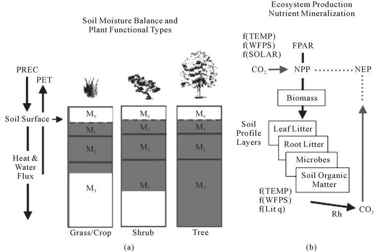
Figure 1. Schematic representation of components in the NASA-CASA model. The soil profile component (a) is layered with depth into a surface ponded layer (M0), a surface organic layer (M1), a surface organic-mineral layer (M2), and a subsurface mineral layer (M3), showing typical levels of soil water content (shaded) in three general vegetation types. The production and decomposition component (b) shows separate pools for carbon cycling among pools of leaf litter, root litter, woody detritus, microbes, and soil organic matter, with dependence on litter quality (Lit q).
gas emissions from vegetation fires, we apply the following equation:
 (2)
(2)
where Et (Pg; 1 Pg = 1015 g) is the regional emissions total at time t (d), B is the biomass subjected to burn at location x, CF is the biomass combustion fraction associated with a particular plant tissue fraction (leaf versus wood), ef is the emission factor (flaming and/or smoldering) associated with a particular trace gas, A is the area burned (km2) at location x and time t.
To estimate the B term in Equation (2), maps of vegetation biomass can be derived by one of two general methods. The first is by spatial interpolation, using what is normally a small number (<100) of intensive field site measurements of aboveground plant mass [28]. A weakness of any interpolation method is that a small number of measurements may not adequately represent the variability of biomass growth patterns. The second general method, and the one used in this study, is developed through our combination of satellite remote sensing and ecosystem carbon flux modeling. Satellite imagery can be transformed using plant production models to provide relatively high spatial resolution maps of above-ground biomass over a regional area of interest [2].
We adopted default CF values largely from the FLAMBE modeling system [29], with several modifications. We used a globally uniform CF value of 0.95 for leaf material [27]. In tropical rainforest zones, we adopted a CF value of 0.45 for wood material, derived from Amazon forest slash burning studies [30,31]. Following the approach of Potter et al. [27], we based these estimates for typical CF values on studies that were conducted in the Amazon on small-holder properties, where all decisions as to which vegetation to burn, size of area slashed, location, and the timing of the slash and burn process (how to slash, how long to dry, when to burn) were entirely left to property owners. The estimated CF values used in our analysis are typical of those reported in several other studies of tropical biomass burning [32].
The ef term in Equation (2) is defined as the amount of a compound released per amount of fuel consumed (g dry matter). Calculation of this parameter requires knowledge of the carbon content of the biomass burned and the carbon budget of the fire usually expressed as the CF term [33]. Where fuel and residue data at the ground level are not available, an overall fuel carbon content of 45% - 50% is commonly assumed [34].
The ef vales we used in Equation (2) were estimated by Scholes et al. [35] based on a review of some 70 publications, a large fraction of which were produced as a result of International Geosphere-Biosphere Programme (IGBP) Biomass Burning Experiment (BIBEX) campaigns. It appears from this compilation of published ef values that adequate data exist for CO2 emissions for savanna and tropical forest fires. Post-disturbance decomposition of residual biomass carbon pools in wood and soils followed the methods of Potter et al. [7].
3.3. Ecosystem Disturbance Events
In this section, we describe algorithms implemented for mapping global land cover change and wildfires based on satellite observations from MODIS data by Mithal et al. [36]. The new forest cover change algorithms were unsupervised in nature and exploit both the temporal and spatial structure in the MODIS data. Using independent wildfire perimeter data sets, we have comprehensively evaluated these algorithms, as well as those from alternate methods, across different forest climatic zones. The framework depends upon the Enhanced Vegetation Index (EVI) from MODIS 16-day Level 3 1 km Vegetation Indices (MOD13A2) products.
The following is a brief description of the algorithms used in this framework for mapping of global forest cover change and wildfires, and subsequently linked to CASA forest biomass pools for carbon emission fluxes. In this stratified framework for mapping forest disturbances, we have employed multiple, complementary scoring mechanisms using 1 km MODIS EVI time series products. The main assumption behind these algorithms is that in mature forests, EVI values for future time steps tend to be similar to previous years when accounting for seasonal variation. On the other hand, changes like wildfires and deforestation are characterized by an abrupt decrease in EVI after the event. The algorithms build a model that is used for predicting the expected EVI values for the future years. Deviation of the future observations from the predicted value indicates a change. A measure that quantities the deviation of future observations from the model prediction is used to assign the change score.
The change score should reflect the significance of deviations with respect to the natural variation of vegetation response for a given forest location. The VID (Vegetation-Independent Yearly Delta) algorithm developed by Mithal et al. [36] addressed this requirement by including the standard deviation of the variability in the change score. It assumed that the random fluctuations in mean annual EVI for a particular vegetation type are normally distributed for a location and estimates the mean (µvar) and standard deviation (∂var) of the variability score distribution as the maximum likelihood estimates for the distribution.
The new VID score was computed as Equation (3):
 (3)
(3)
Mithal et al. [36] examined the performance of the new VID forest disturbance algorithm in several regions around the world, including the states of California (US) and the Yukon (Canada). Results demonstrated high accuracy levels for all major wildfires mapped from aerial surveys in these diverse forest regions. Mithal et al. [36] quantitatively showed that the VID forest change algorithms perform better than the well-known MODIS burned area (BA) framework [37] in the state of California (US) and were comparable in results to the BA framework for wildfire disturbances in the Yukon (Canada).
4. Results
4.1. CASA Validation with Tower Flux Measurements
Flux estimates from eddy-correlation analysis were obtained from AmeriFlux tower flux sites that could meet certain criteria for CASA model comparisons. First, at least three complete years of site flux measurements were required to evaluate model predictions of interannual variations in CASA NEP fluxes. Second, winter (and/or dormant/dry) season NEP fluxes were required from a site to evaluate model predictions of soil CO2 emissions on a year-round basis. Third, tower sites were required to be representative of the predominant vegetation class setting in the global land cover data used as input to the CASA model.
For sites meeting all of these criteria, AmeriFlux data sets were obtained from the central data repository located at the Carbon Dioxide Information Analysis Center (CDIAC; public.ornl.gov/ameriflux/dataproducts.shtml). Level 4 AmeriFlux records contained gap-filled and µstar filtered records, complete with calculated gross productivity and total ecosystem respiration terms on varying time intervals including hourly, daily, weekly, and monthly with flags for the quality of the original and gapfilled data.
CASA monthly NEP predictions from the MOD13C2 EVI data values closest to the tower location were compared to AmeriFlux eddy-correlation monthly estimates of the corresponding NEP fluxes. We note that the monthly MODIS EVI values in practically every grid cell of the global CASA model will be influenced by periodic land cover disturbances and (some naturally occurring) areas of sparse vegetation cover, including development, roads, water bodies. It was expected, therefore, that CASA model NEP flux predictions would be systematically lower than tower measurements of these carbon fluxes, since tower footprints tend to be far less affected by wildfire and other disturbances (such as logging and forest thinning), compared for instance to the surrounding MODIS grid cell area in which they are located.
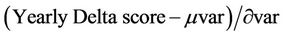
A total of four AmeriFlux tower sites, together reporting 196 monthly measurements, were found to meet the criteria cited above for comparison to CASA model NEP predictions (Figure 2). CASA model predictions closely followed the seasonal timing of AmeriFlux tower measurements at each site. The linear regression correlation coefficient between CASA NEP predictions and tower fluxes was estimated at R2 = 0.41 (p < 0.05) for all sites combined. Most of the unexplained variance in this model-to-tower flux comparison resulted from the Blodgett evergreen needle-leaf forest tower site, which showed a sudden shift upwards in NEP (greatly enhanced ecosystem carbon sink) after 2001 in the AmeriFlux data sets, presumably due to stand thinning in 2000 [38]. We note that Tang et al. [39] reported a similar correlation value (R2 = 0.45) in model-to-tower NEP flux comparesons at the Blodgett forest location, compared to higher correlations (all with R2 > 0.50) at seven other AmeriFlux forest sites, which implied that small-scale forest management at the Blodgett site is an unaccounted source of uncertainty in our model flux comparisons.
4.2. Global Net Primary Production
As previously reported by Potter et al. [13], predicted terrestrial NPP for the globe in 2009 was 50.1 Pg C, a total carbon flux in the middle of the range of previous vegetation NPP predictions of between 44 to 66 Pg C per year for the period 1982-1998 [40,41]. We estimate that global terrestrial NPP increased by +0.14 Pg C over the time period of 2000 to 2009, due almost entirely to a strong upward trend in the Northern Hemisphere (Figure 3). Annual NPP was predicted to have increased between the years 2000 and 2007 in the regions of high-latitude (>50˚N) North America and Eurasia, and also in South Asia, West and Central Africa, and the western Amazon. This upward trend in high-latitude NPP was controlled by a combination of rapidly warming temperatures from 2004 to 2005 and by elevated MODIS EVI patterns, which in turn were closely correlated with precipitation amounts [13]. Periodic declines in regional NPP levels were predicted for the southern Untied States, the southern Amazon, western Europe, southern and eastern Africa, and Australia; the timing of negative NPP anomalies in each of these regions was associated with severe droughts and, in some cases, extreme heat waves [42].
4.3. Global Net Ecosystem Production
Subtracting monthly Rh fluxes from monthly NPP fluxes yields NEP flux estimates. Predicted global NEP fluxes from 2000 through 2005 showed a roughly balanced terrestrial biosphere carbon cycle, with variations less than ±0.5 Pg C yr−1 (Figure 4). Nonetheless, beginning in 2006, global NEP fluxes became increasingly imbalanced, starting from −0.9 Pg C yr−1 to the largest negative (net terrestrial source) flux of −2.2 Pg C yr−1 in 2009. Notable surface temperature warming from 2000-2005
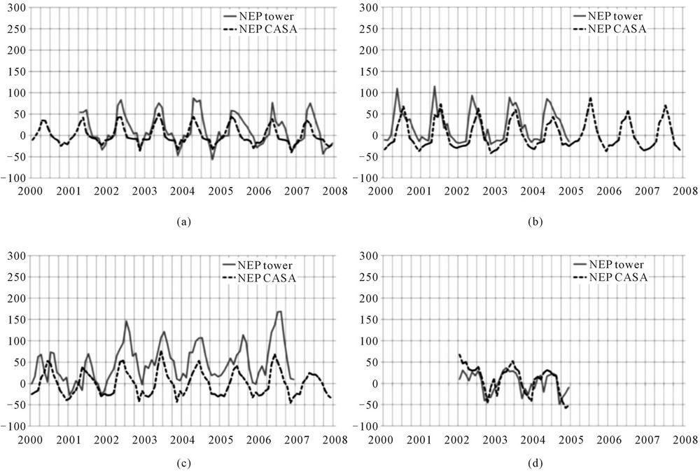
Figure 2. Comparison of CASA monthly NEP to Ameriflux measurements derived from eddy-correlation estimates of the corresponding monthly fluxes. (a) Tonzi savanna grassland; (b) Howland mixed forest; (c) Blodgett evergreen needle-leaf forest; (d) Tapajos evergreen broad-leaf forest.

Figure 3. Spatial pattern of terrestrial NPP linear trends from 2000 through 2009.
was significantly associated with positive NEP (net sink) fluxes in high northern latitude tundra, grasslands, and boreal forest areas, whereas from 2005-2009, major drought events were associated with negative NEP (net source fluxes) in tropical evergreen forests, temperate deciduous forests, croplands, grasslands, and savannas worldwide (Figure 5).
Above average temperatures across the high latitude

Figure 4. Interannual variations from 2000 through 2009 in anomalies of annual total NEP for the CASA model for the Northern Hemisphere (NH-green circles) and the Southern Hemisphere (SH-red circles). Units are Pg C yr−1 (1 Pg = 1015 g), with positive values indicating net ecosystem sink fluxes and negative values indicating net ecosystem source fluxes.
zones of eastern Canada and Eurasia (World Meteorological Organization, [42]) corresponded to positive NEP (net sink fluxes) from the CASA model. Extreme heat waves were reported across Central Asia, the United States, and China from 2000 to 2002. In 2003, much of
Figure 5. Global predicted NEP fluxes from (a) 2003 (highest total ecosystem sink flux) and (b) 2009 (highest total ecosystem source flux). Units are g C m−2 yr−1 gridded at 0.5 deg spatial resolution.
Europe, Canada, Russia, and China experienced summer periods of warming temperatures. From 2004 to 2008, parts of Pakistan, Australia, the United States, Canada, and Europe continued to experience extreme heat waves. On the other hand, extreme cold winter temperatures were reported repeatedly in Russia, India, and China over the period 2000 to 2008. Large parts of Europe experienced unusually cold temperatures in the summer of 2001, as did Australia and South Africa in 2007.
There were many instances of severe drought across the globe during the period of 2000 to 2008, mainly affecting regions of the central North America, Africa, Brazil, and China (World Meteorological Organization, [42]). Beginning with major droughts in Brazil, the Horn of Africa, the Middle East, Central and South Asia, and China in 2000 and 2001, these events were followed by most of North America, southern Africa, and Australia experiencing record low precipitation amounts in 2002, 2003, and 2004. Large areas of Europe, southern Africa, Brazil, and Paraguay were affected by severe droughts in 2005. From 2006 though 2008, much of the United States, eastern and southern Africa, China, and Australia experienced continued deficits of precipitation. Strongly negative NEP fluxes were predicted to be associated with droughts reported in South Asia, eastern Africa, northern China, and northern and eastern coastal South America. Strongly positive NEP fluxes predicted by the CASA model were associated with periodically heavy rainfall amounts in Eastern Europe, Siberia, Australia, West Africa, and southern Africa.
4.4. Ecosystem Disturbance Emissions
Comparison of areas of disturbed forest land between CASA model inputs and national reports from the Food and Agriculture Organization [43] of the United Nations showed a close match among the 30 leading counties in terms of hectares of forest converted (Table 1). Six of the top ten counties ranked by the FAO in terms of annual forest conversion rates (2005-2009) were also among the top ten counties mapped for forest lands converted in our CASA model inputs from 2005-2009 MODIS data. The notable exceptions in the global comparison shown in Table 1 were that of India and Papua New Guinea (FAO ranks 3 and 6, respectively). These two Asian countries were still ranked among the 30 leading counties for forest area converted in CASA model inputs. According to the FAO [43], India recorded over 25 million hectares of forests as being affected by grazing by domestic animals, a cover change that involves the type of gradual forest degradation processes that are difficult to detect by satellite remote sensing from MODIS.
CASA model predictions of CO2 emissions from forest disturbance and biomass burning (Figure 6) were highest on a unit area (g C m−2 yr−1) basis in the region of Southeast Asia (specifically in the countries of Myanmar, Malaysia, Cambodia, Vietnam, and Indonesia). Although the CO2 emissions on a unit area basis from forest disturbance in the United States and Brazil were estimated at less than half of those estimated from Southeast Asian countries (Table 2), the total areas of forest disturbed annually gave the United States and Brazil the highest national totals of carbon lost from biomass burning in 2009. Forested regions of the Pacific Northwest, the southeastern US and Gulf Coast, and the Amazon rainforest were consequently major contributors to global biomass emissions to the atmosphere (Figure 6).
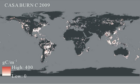
Figure 6. Global predicted biomass burning fluxes of CO2 in 2009. Units are g C m−2 yr−1 gridded at 0.5 degree spatial resolution.
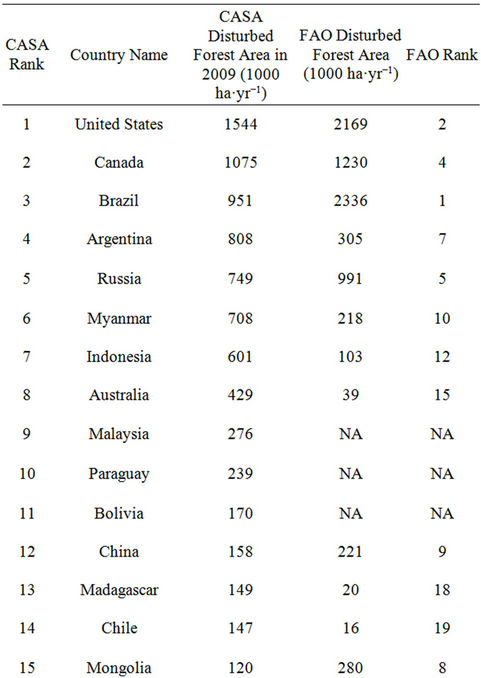
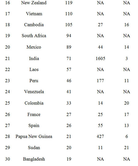
Table 1. Comparison of area forest disturbed between CASA model inputs and FAO reported statistics by country from 2005-2010 (FAO, 2010).
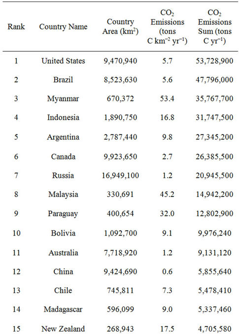
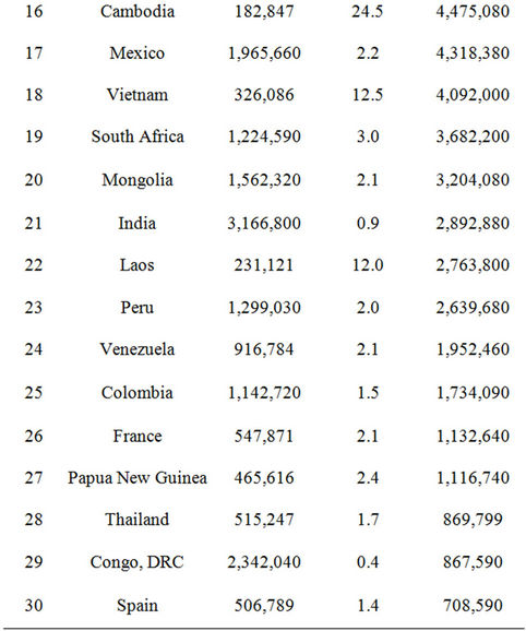
Table 2. Countries ranked in terms of carbon emissions from forest disturbance and biomass burning from the CASA model in 2009.
The global sum of CO2 emissions from forest disturbance and biomass burning for 2009 alone was predicted at 0.51 Pg C yr−1. Decomposition emissions of residual (dead) forest biomass in the CASA model from three years (2007 to 2009) of deforestation globally added 0.15 Pg C yr−1 to the atmosphere.
5. Discussion
A recent study by Zhao and Running [19] reported a decreasing trend in global terrestrial NPP from 2000 to 2009, using MODIS satellite inputs and the same NCEP reanalysis data set as in the CASA model for climate inputs. On a regional basis, our CASA model results differed from Zhao and Running [19] which reported that NPP in the tropical zones (23.5˚S to 23.5˚N) explained 93% of variations in the global NPP. In contrast, we found that NPP in the tropical zones explained only 50% - 60% of variations in the global NPP, whereas NPP in the latitude zone between 30˚N and 60˚N could explain between 40% and 50% of variations in the global NPP [13]. Notwithstanding the difference in the global trend of NPP between CASA and the predictions from Zhao and Running [19] the overall patterns of interannual variations in Northern and Southern Hemisphere NPP anomalies were similar between the two model results. NPP anomalies in the Northern Hemisphere were negative from 2000-2003 and then became strongly positive from 2004-2008, closely following the 0.1˚ yr−1 surfacewarming trend in the model input data. NPP anomalies in the Southern Hemisphere were positive from 2000-2003 and then turned negative between 2004-2008, with 2005 being the most strongly negative anomaly year.
The more complete CASA model NEP results reported in this paper suggest that surface temperature warming together with regional droughts (e.g., from 2006 to 2009) can drive ecosystem carbon losses to the atmosphere of more than 1 Pg C yr−1 in excess of long-term average terrestrial NEP fluxes. These predicted changes in NEP fluxes over a decade of model results would have made a larger impact on atmospheric CO2 concentrations than NPP trends alone, and our results highlight the importance of including the annual variations in soil Rh decomposition fluxes from downed and burned plant biomass in global carbon cycle. Variations in plant production alone can account for less than one-third of terrestrial ecosystem fluxes in most years.
The forest fire and land cover change mapping framework presented in this paper has limitations under several scenarios. These include situations where 1) the vegetation rapidly recovers after a fire or if there are multiple fires in rapid succession; 2) the loss in vegetation green cover associated with land cover conversion is insignificant, such as in crop fallow and rotation practices; 3) the vegetation cover has high natural variability in seasonal greenness, which is common in mixed woodland-grassland ecosystems. Each of these scenarios poses distinct challenges for our current land cover change detection framework that are being addressed in future validation studies with extensive ground-truth data sets.
Nevertheless, we have identified numerous relatively small-scale patterns throughout the world where terrestrial carbon fluxes may vary between net annual sources and sinks from one year to the next. We conclude that accurately monitoring of NEP for these areas of high interannual variability will require further validation of carbon model estimates, with a focus on both flux algorithm mechanisms and potential scaling errors to the regional level.
6. Acknowledgements
This work was supported by funding from the NASA Carbon Monitoring System program, the Planetary Skin Institute, and NSF Grant IIS-0905581 and NSF Grant IIS-1029711 to Vipin Kumar at the University of Minnesota.
REFERENCES
- R. A. Houghton, “The Annual Net Flux of Carbon to the Atmosphere from Changes in Land Use 1850-1990,” Tellus, Vol. 51(B), 1999, pp. 298-313.
- C. S. Potter, “Terrestrial Biomass and the Effects of Deforestation on the Global Carbon Cycle,” BioScience, Vol. 49, No. 10, 1999, pp. 769-778. doi:10.2307/1313568
- P. M. Fearnside, “Global Warming and Tropical Land- Use Change: Greenhouse Gas Emissions from Biomass Burning, Decomposition and Soils in Forest Conversion, Shifting Cultivation and Secondary Vegetation,” Climatic Change, Vol. 46, No. 1-2, 2000, pp. 115-158. doi:10.1023/A:1005569915357
- A. D. McGuire, S. Sitch and J. S. Clein, “Carbon Balance of the Terrestrial Biosphere in the Twentieth Century: Analyses of CO2, Climate and Land Use Effects with Four Process-Based Ecosystem Models,” Global Biogeochemical Cycles, Vol. 15, No. 1, 2001, pp. 183-206. doi:10.1029/2000GB001298
- R. S. DeFries, R. A. Houghton and M. C. Hansen, “Carbon Emissions from Tropical Deforestation and Regrowth Based on Satellite Observations for the 1980s and 1990s,” Proceedings of the National Academy of Science USA, Vol. 99, 2002, pp. 14256-14261. doi:10.1073/pnas.182560099
- F. Achard, H. D. Eva, P. Mayaux, J. Stibig and A. Belward, “Improved Estimates of Net Carbon Emissions from Land Cover Change in the Tropics for the 1990s,” Global Biogeochemical Cycles, Vol. 18, No. 2, 2004, 11 p.
- C. S. Potter, S. Klooster and V. Genovese, “Carbon Emissions from Deforestation in the Brazilian Amazon Region,” Biogeosciences, Vol. 6, No. 11, 2009, pp. 2369- 2381. doi:10.5194/bg-6-2369-2009
- N. Ramankutty, H. K. Gibbs, F. Achard, R. Defries, J. A. Foley and R. A. Houghton, “Challenges to Estimating Carbon Emissions from Tropical Deforestation,” Global Change Biology, Vol. 13, No. 1, 2007, pp. 51-66. doi:10.1111/j.1365-2486.2006.01272.x
- C. S. Potter, J. T. Randerson, C. B. Field, P. A. Matson, P. M. Vitousek, H. A. Mooney and S. A. Klooster, “Terrestrial Ecosystem Production: A Process Model Based on Global Satellite and Surface Data,” Global Biogeochemical Cycles, Vol. 7, No. 4, 1993, pp. 811-841. doi:10.1029/93GB02725
- A. Huete, K. Didan, T. Miura and E. Rodriguez, “Overview of the Radiometric and Biophysical Performance of the MODIS Vegetation Indices.” Remote Sensing of Environment, Vol. 83, 2002, pp. 195-213. doi:10.1016/S0034-4257(02)00096-2
- A. Huete, K. Didan, Y. E. Shimabukuro, P. Ratana, S. R. Saleska, L. R. Hutyra, D. Fitzjarrald, W. Yang, R. R. Nemani and R. Myneni, “Amazon Rainforests Green-Up with Sunlight in Dry Season,” Geophysical Research Letters, Vol. 33, 2006, Article ID: L06405. doi:10.1029/2005GL025583
- C. Potter, S. Klooster, R. Myneni, V. Genovese, P. Tan and V. Kumar, “Continental Scale Comparisons of Terrestrial Carbon Sinks Estimated from Satellite Data and Ecosystem Modeling 1982-1998,” Global and Planetary Change, Vol. 39, 2003, pp. 201-213. doi:10.1016/j.gloplacha.2003.07.001
- C. Potter, S. Klooster and V. Genovese, “Net Primary Production of Terrestrial Ecosystems from 2000 to 2009,” Climatic Change, Vol. 113, 2012, pp. 1-13. doi:10.1007/s10584-012-0460-2
- X. Xiao, S. Hagen, Q. Zhang, M. Keller and B. Moore III, “Detecting Leaf Phenology of Seasonally Moist Tropical Forests in South America with Multi-Temporal MODIS Images,” Remote Sensing of Environment, Vol. 103, No. 4, 2006, pp. 465-473. doi:10.1016/j.rse.2006.04.013
- R. R. Colditz, C. Conrad, T. Wehrmann, M. Schmidt and S. W. Dech, “Analysis of the Quality of Collection 4 and 5 Vegetation Index Time Series from MODIS,” ISPRS Spatial Data Quality Symposium, CRC press, Enschede, 2007.
- J. L. Monteith, “Solar Radiation and Productivity in Tropical Ecosystems,” Journal of Applied Ecology, Vol. 9, No. 3, 1972, pp. 747-766. doi:10.2307/2401901
- R. J. Olson, J. M. O. Scurlock, W. Cramer, W. J. Parton and S. D. Prince, “From Sparse Field Observations to a Consistent Global Dataset on Net Primary Production,” IGBP-DIS Working Paper No. 16, IGBP-DIS, Toulouse, 1997.
- R. Kistler, E. Kalnay, W. Collins, S. Saha, G. White, J. Woollen, M. Chelliah, W. Ebisuzaki, M. Kanamitsu, V. Kousky, H. van den Dool, R. Jenne and M. Fiorino, “The NCEP-NCAR 50-Year Reanalysis: Monthly Means CDROM and Documentation,” Bulletin of the American Meteorological Society, Vol. 82, No. 2, 2001, pp. 247-268. doi:10.1175/1520-0477(2001)082<0247:TNNYRM>2.3.CO;2
- M. Zhao and S. W. Running, “Drought-Induced Reduction in Global Terrestrial Net Primary Production from 2000 through 2009,” Science, Vol. 329, No. 5994, 2010, pp. 940-943. doi:10.1126/science.1192666
- C. H. B. Priestly and R. J. Taylor, “On the Assessment of Surface Heat Flux and Evaporation Using Large-Scale Parameters,” Monthly Weather Review, Vol. 100, No. 2, 1972, pp. 81-92. doi:10.1175/1520-0493(1972)100<0081:OTAOSH>2.3.CO;2
- D. C. Nepstad, C. R. de Carvalho, E. A. Davidson, P. H. Jipp, P. A. Lefebvre, G. H. Negreiros, E. D. da Silva, T. A. Stone, S. E. Trumbore and S. Vieira, “The Role of Deep Roots in the Hydrological and Carbon Cycles of Amazonian Forests and Pastures,” Nature, Vol. 372, No. 6507, 1994, pp. 666-669. doi:10.1038/372666a0
- X. Xiao, Q. Zhang, S. R. Saleska, L. Hutyra, P. Camargo, S. Wofsy, S. Frolking, S. Boles, M. Keller and B. Moore III, “Satellite-Based Modeling of Gross Primary Production in a Seasonally Moist Tropical Evergreen Forest,” Remote Sensing of Environment, Vol. 94, 2005, pp. 105-122. doi:10.1016/j.rse.2004.08.015
- K. Ichii, H. Hashimoto, M. A. White, C. Potter, L. R. Hutyra, A. R. Huete, R. B. Myneni and R. R. Nemani, “Constraining Rooting Depths in Tropical Rainforests Using Satellite Data and Ecosystem Modeling for Accurate Simulation of GPP Seasonality,” Global Change Biology, Vol. 13, No. 1, 2007, pp. 67-77. doi:10.1111/j.1365-2486.2006.01277.x
- A. R. Jumikis, “Thermal Soil Mechanics,” Rutgers University Press, New Brunswick, 1966.
- G. B. Bonan, “A Computer Model of the Solar Radiation, Soil Moisture and Soil Thermal Regimes in Boreal Forests,” Ecological Modelling, Vol. 45, No. 4, 1989, pp. 275-306. doi:10.1016/0304-3800(89)90076-8
- B. Walker and W. Steffen, “An Overview of the Implications of Global Change for Natural and Managed Terrestrial Ecosystems,” Conservation Ecology, Vol. 1, No. 2, 1997, pp. 2-17.
- C. S. Potter, V. Brooks-Genovese, S. Klooster and A. Torregrosa, “Biomass Burning Emissions of Reactive Gases Estimated from Satellite Data Analysis and Ecosystem Modeling for the Brazilian Amazon Region,” Journal of Geophysical Research, Vol. 107, No. D20, 2002, pp. 8056-8066. doi:10.1029/2000JD000250
- R. A. Houghton, D. L. Skole, C. A. Nobre , J. L. Hackler, K. T. Lawrence and W. H. Chomentowski, “Annual Fluxes of Carbon from Deforestation and Regrowth in the Brazilian Amazon,” Nature, Vol. 403, No. 6767, 2000, pp. 301-304. doi:10.1038/35002062
- J. S. Reid, E. J. Hyer, E. M. Prins, D. L. Westphal, J. Zhang, J. Wang, S. A. Christopher, C. A. Curtis, C. C. Schmidt, D. P. Eleuterio, K. A. Richardson and J. P. Hoffman, “Global Monitoring and Forecasting of Biomass-Burning Smoke: Description of and Lessons from the Fire Locating and Modeling of Burning Emissions (FLAMBE) Program,” IEEE Journal of Selected Topics in Applied Earth Observations and Remote Sensing, Vol. 3, No. 2, 2009, pp. 144-162. doi:10.1109/JSTARS.2009.2027443
- J. B. Kauffman, D. L. Cummings, D. E. Ward and R. Babbitt, “Fire in the Brazilian Amazon: Biomass, Nutrient Pools, and Losses in Slashed Primary Forests,” Oecologia, Vol. 104, No. 4, 1995, pp. 397-408. doi:10.1007/BF00341336
- C. L. Sorrensen, “Linking Smallholder Land Use and Fire Activity: Examining Biomass Burning in the Brazilian Lower Amazon,” Forest Ecology and Management, Vol. 128, No. 1, 2000, pp. 11-25. doi:10.1016/S0378-1127(99)00283-2
- W. M. Hao and M.-H. Lui, “Spatial and Temporal Distribution of Tropical Biomass Burning,” Global Biogeochemical Cycles, Vol. 8, No. 4, 1994, pp. 495-503. doi:10.1029/94GB02086
- D. E. Ward, W.-M. Hao, R. A. Susott, R. A. Babbitt, R. W. Shea, J. B. Kauffman and C. O. Justice, “Effect of Fuel Composition on Combustion Efficiency and Emission Factors for African Savanna Ecosystems,” Journal of Geophysical Research, Vol. 101, No. D19, 1996, pp. 23569-23576. doi:10.1029/95JD02595
- W. Seiler and P. J. Crutzen, “Estimates of Gross and Net Fluxes of Carbon between the Biosphere and the Atmosphere from Biomass Burning,” Climatic Change, Vol. 2, 1980, pp. 207-247. doi:10.1007/BF00137988
- M. Scholes, P. Matrai, K. Smith, M. Andreae and A. Guenther, “Biosphere-Atmosphere Interactions, in Atmospheric Chemistry in a Changing World,” Cambridge University Press, New York, 2000.
- V. Mithal, A. Garg, I. Brugere, S. Boriah, V. Kumar, M. Steinbach, C. Potter and S. A. Klooster, “Incorporating Natural Variation into Time Series-Based Land Cover Change Detection,” Proceedings of the 2011 NASA Conference on Intelligent Data Understanding, Mountain View, 19-21 October 2001, pp. 45-59.
- C. O. Justice, L. Giglio, D. Roy, L. Boschetti, I. Csiszar, D. Davies, S. Korontzi, W. Schroeder, K. O’Neal and J. Morisette, “MODIS-Derived Global Fire Products,” In: B. Ramachandran, C. O. Justice and M. J. Abrams, Eds., Land Remote Sensing and Global Environmental Change, Springer, Berlin, 2011, pp. 661-679.
- L. Misson, J. Tang, M. Xu, M. McKay and A. Goldstein, “Influences of Recovery from Clear-Cut, Climate Variability, and Thinning on the Carbon Balance of a Young Ponderosa Pine Plantation,” Agricultural and Forest Meteorology, Vol. 130, 2005, pp. 207-222. doi:10.1016/j.agrformet.2005.04.001
- X. Tang, Z. Wang, D. Liu, K. Song, M. Jia, Z. Dong, J. W. Munger, D. Y. Hollinger, P. V. Bolstad, A. H. Goldstein, A. R. Desai, D. Dragoni and X. Liu, “Estimating the Net Ecosystem Exchange for the Major Forests in the Northern United States by Integrating MODIS and AmeriFlux Data,” Agricultural and Forest Meteorology, Vol. 156, 2012, pp. 75-84. doi:10.1016/j.agrformet.2012.01.003
- W. Cramer, D. W. Kicklighter, A. Bondeau, B. Moore, G. Churkina, B. Nemry, A. Ruimy and A. L. Schloss, “Comparing Global Models of Terrestrial Net Primary Productivity (NPP): Overview and Key Results,” Global Change Biology, Vol. 5, 1999, pp. 1-15. doi:10.1046/j.1365-2486.1999.00009.x
- R. R. Nemani, C. D. Keeling, H. Hashimoto, W. M. Jolly, S. C. Piper, C. J. Tucker, R. B. Myneni and S. W. Running, “Climate Driven Increases in Global Terrestrial Net Primary Production from 1982 to 1999,” Science, Vol. 300, No. 5625, 2003, pp. 1560-1563. doi:10.1126/science.1082750
- World Meteorological Organization, “WMO Statement on the Status of the Global Climate in 2001,” WMO#670, 2001.
- Food and Agriculture Organization (FAO) of the United Nations, “Global Forest Resource Assessment, FAO Forestry Paper 163,” Rome, 2010, 340 p.