Journal of Flow Control, Measurement & Visualization
Vol.1 No.2(2013), Article ID:34563,8 pages DOI:10.4236/jfcmv.2013.12009
Reconstruction of the Unsteady Supersonic Flow around a Spike Using the Colored Background Oriented Schlieren Technique
1French-German Research Institute of Saint-Louis (ISL), Saint-Louis, France
2Graduate School of Engineering Chiba University, Chiba, Japan
Email: friedrich.leopold@isl.eu
Copyright © 2013 Friedrich Leopold et al. This is an open access article distributed under the Creative Commons Attribution License, which permits unrestricted use, distribution, and reproduction in any medium, provided the original work is properly cited.
Received March 6, 2013; revised May 1, 2013; accepted June 5, 2013
Keywords: Unsteady Spike Flow; Reconstruction; Density Field; Schlieren Technique
ABSTRACT
In this paper, the improved Background Oriented Schlieren technique called CBOS (Colored Background Oriented Schlieren) is described and used to reconstruct the density fields of three-dimensional flows. The Background Oriented Schlieren technique (BOS) allows the measurement of the light deflection caused by density gradients in a compressible flow. For this purpose the distortion of the image of a background pattern observed through the flow is used. In order to increase the performance of the conventional Background Oriented Schlieren technique, the monochromatic background is replaced by a colored dot pattern. The different colors are treated separately using suitable correlation algorithms. Therefore, the precision and the spatial resolution can be highly increased. Furthermore a special arrangement of the different colored dot patterns in the background allows astigmatism in the region with high density gradients to be overcome. For the first time an algebraic reconstruction technique (ART) is then used to reconstruct the density field of unsteady flows around a spike-tipped model from CBOS measurements. The obtained images reveal the interaction between the free-stream flow and the high-pressure region in front of the model, which leads to large-scale instabilities in the flow.
1. Introduction
For the investigation of compressible flows the determination of the density distribution is of prime importance. For this purpose, the schlieren method, introduced by A. Toepler in 1864, is currently used [1]. The schlieren technique transforms the phase variation of the light passing through a phase object into an intensity variation. Other techniques such as the density speckle photography appeared in the seventies and allowed the direct measurement of the deflection of the light [2,3]. Later, Wernekink and Merzkirch [4] and Niessen et al. [5] used an improved version of the density speckle photography for this purpose.
The Background Oriented Schlieren (BOS) technique is based on a patent held by Meier [6] and more precisely described by Raffel et al. [7,8]. In order to measure the light deflection caused by density gradients in a compressible flow, the BOS technique uses the distortion of a background image. Tiny, randomly distributed dots on a flat plate are used as a background. The recording has to be performed as follows: first a reference image is generated by recording the background pattern observed through the air at rest before or after the experiment. Secondly, an additional exposure through the flow under investigation leads to a displaced image of the background pattern. The resulting images of both exposures can then be evaluated by correlation methods, leading to the local displacements related to the deviations of the rays. This paper describes how to improve the accuracy of the BOS technique and how to treat strong density gradients causing blurred images by using a background with colored dots and suitable correlation algorithms (CBOS technique).
Furthermore, the measured displacements of the rays are a projection of the gradients of the density field in a given observation direction. By using multiple projection data the three-dimensional density distribution of a flow field can be reconstructed, for example, with Computed Tomography (CT). An axisymmetric flow density distribution can be obtained with techniques based on the Abel or the Fourier transforms, as shown by Venkatakrishnan et al. [9,10], Sourgen et al. [11] and Kak et al. [12]. In the papers by Ota et al. [13,14] the Algebraic Reconstruction Technique (ART) is also shown to be suitable in the reconstruction of density fields, especially for the case where the flow around a model has to be reconstructed.
Former studies about spike-tipped models pointed out [15-18] the interaction between the incoming free stream flow and the high-pressure region near the model, which could have an influence on upstream at the tip of the spike by displacing the boundary layer along the spike and subsequently inducing a large-scale instability of the flow. In this paper, the unsteady flow around a spiketipped model at Mach number 3 is studied. Therefore a high-speed camera is used. Supposing the flow to be axially symmetrical, an algebraic reconstruction technique (ART) is applied to reconstruct the density field around the spike.
2. Background Oriented Schlieren Technique (BOS)
2.1. Principles of the BOS
The principle of the BOS technique is based on the measurement of the deviation of the light passing through a phase object. Indeed, the BOS technique uses the distortion of a background image for detecting the changes in density gradients. Thanks to the empirical law of Gladstone-Dale, the density can directly be related to the refractive index:
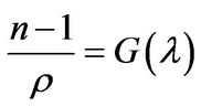 (1)
(1)
where n denotes the refractive index which is defined as the ratio of the speed of light in vacuum to the speed of light in the optical medium; ρ stands for the density of the medium, G denotes the Gladstone-Dale constant which depends on the characteristics of the gas and λ represents the wavelength of the light. As the changes in the Gladstone-Dale constant in the visible spectral range are very small, the constant is set to the value
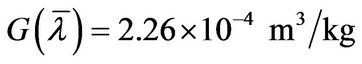 for an average wavelength of λ ≈ 550 nm. The distortion χ can be expressed by integrating the local index gradients along the light path:
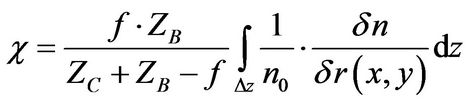 (2)
(2)
where z represents the coordinate along the light path, f the focal length of the camera lens, ZC the distance from the camera to the phase object and ZB the distance from the phase object to the background image, as shown in Figure 1. Now the Gladstone-Dale relation allows us to draw conclusions from the two-dimensional distortion χ(x,y) in order to determine the density gradients  and
and  in the horizontal and vertical directions, respectively [8].
2.2. The Color Distribution in the Background Image
The CBOS technique normally uses a computer-generated random dot pattern which is placed in the background of the test volume. This pattern has to possess a high spatial frequency that can be imaged with a high contrast. It usually consists of tiny, randomly distributed dots. Earlier studies [11,19] pointed out that the dot pattern for an optimized evaluation should cover from 30% to 70% of the surface of the background image.
Since the primary colors red, green and blue (according to the RGB color model) can easily be detected by commercial digital CMOS cameras, these colors are used to generate the colored background for the CBOS technique. The background pattern is assembled as follows: the same proportion of each primary color is distributed randomly over the background image. This leads to a specific distribution of pure and compound colors over the background (Figure 2). It can be observed that a filling rate of 35% for each primary color leads to a maximum distribution of the pure colors. Furthermore, the distribution of the compound colors and of the uncolored areas is close to 30%. A typical colored background image is shown in Figure 3 with a filling rate of 35% for each primary color [19].
2.3. Image Processing
In order to improve the analysis of the recorded images,
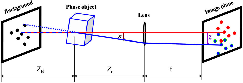
Figure 1. Optical setup for the BOS technique.
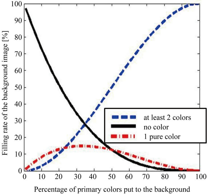
Figure 2. Distribution of the compound colors as a function of the primary color filling rate.
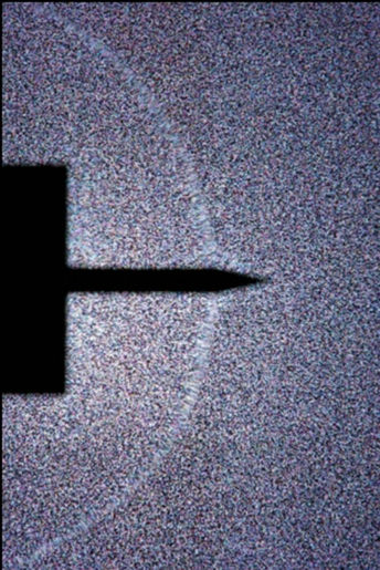
Figure 3. Spike-tipped model in front of the colored background at Mach number 3.
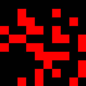
the post processing takes into account the fact that digital CMOS cameras have sensors for the primary colors, i.e. red, green and blue. The data from the sensors are directly stored without any treatment or compression, using a special raw format. Due to the decomposition into the three primary colors, 8 elementary dot patterns can be extracted from the image (Figure 4):
• one pattern for each of the primary colors (red, green and blue);
• one pattern for all secondary colors;
• 3 patterns of dots containing red, green and blue, respectively; and
• one pattern for the uncolored areas, the so-called “black dots”.
The assessment of the image distortion is achieved by treating each of the 8 elementary patterns separately by means of the cross-correlation method already applied in the PIV technique [20-23]. In order to increase the preci-
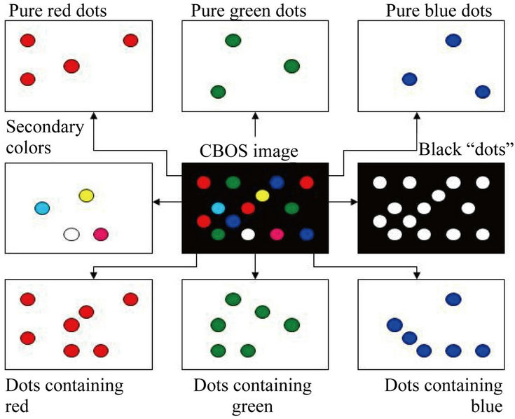
Figure 4. Extraction of the 8 elementary dot patterns from the colored background image.
sion of the common BOS technique, an ensemble averaging of the cross-correlations for all 8 dot patterns at each location is performed. The standard error of the mean for the eight dot patterns is smaller than  of the standard variation for a black and white background, which leads to a relative error of 0.7% for a displacement of 5 pixels (Figures 5-10). More details about the comparison with the BOS technique can be found in [19]. Finally an average value for each location is determined by the value obtained at the location itself and by the results from interpolations between the opposite neighboring values. In order to increase the accuracy of the measurement, the values used for the averaging process must satisfy a standard deviation criterion.
In regions with high density gradients, e.g. shock waves, the image of the dots is completely blurred due to astigmatism (Figure 11). In order to overcome this problem, the red dot pattern (Figure 12(a)) is shifted in the horizontal direction and colored in green (Figure 12(b)). In a second step the same red dot pattern is shifted in the vertical direction and colored in blue (Figure 12(c)). In these regions where the blurred image of the dots appears, the usual CBOS processing does not work. Therefore, the horizontal displacements are determined by cross-correlations between the red and green dot patterns and the vertical displacements are determined by cross-correlations between the red and blue dot patterns, respectively.
3. Wind-Tunnel Tests
The experiments are carried out in the 0.2 m ´ 0.2 m supersonic blow-down wind tunnel of ISL with a freestream Mach number of 3. The Reynolds number ReD based on the model diameter (D = 40 mm) is 2.7 ´ 106; the tunnel freestream static pressure p is 190 hPa and the
 (a)
(a) (b)
(b) (c)
(c) (d)
(d)
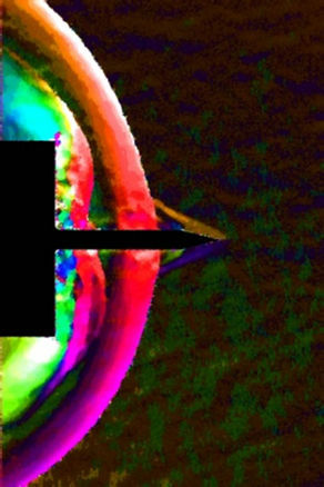
Figure 5. Flow visualization around the spike at t = 0 μs. (a) Pseudo color schlieren for the displacements; (b) Horizontal displacements; (c) Vertical displacements; (d) Isosurface for the density value ρ/ρ∞ = 1.75 in front of the cylinder.
 (a)
(a)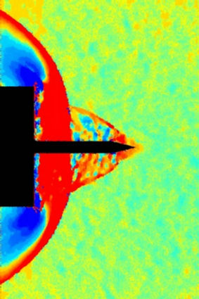 (b)
(b)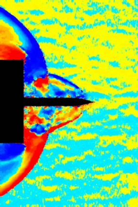 (c)
(c)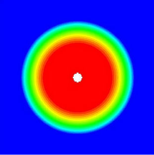 (d)
(d)
Figure 6. Flow visualization around the spike at t = 74 μs. (a) Pseudo color schlieren for the displacements; (b) Horizontal displacements; (c) Vertical displacements; (d) Radial distribution of the density in front of the cylinder (4 mm).
 (a)
(a)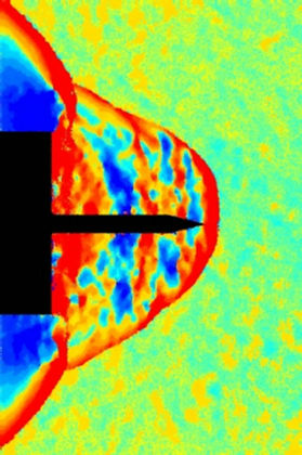 (b)
(b)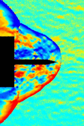 (c)
(c)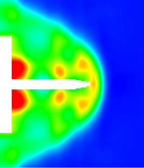 (d)
(d)
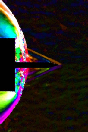
Figure 7. Flow visualization around the spike at t = 148 μs. (a) Pseudo color schlieren for the displacements; (b) Horizontal displacements; (c) Vertical displacements; (d) Reconstructed density on a midplane.
freestream density ρ is 0.651 kg∙m−3. The test models used for this investigation have a cylindrical centerbody mounted on a sting assembly along the wind-tunnel centerline. The angle of attack is set to zero. The spike at the front of the model is l = 35 mm long and the nose is a cone with a half-angle of 14˚ (Figure 3).
The optical setup is built perpendicularly to the symmetry line of the model. The CBOS images are recorded with a Phantom v1610 high-speed camera with 27,000 fps (frames per second). The exposure time is 36 μs. Due to this high frequency the size of the images is 640 ´ 800 pixels. The background is illuminated by a continuous white light source. The reconstruction of the density field is based on the pictures from the high speed camera. In order to increase the depth of field and the accuracy of the CBOS measurement, a telecentric optical system (Figure 13) is introduced, as described by Ota et al. [24]. Furthermore, complementary images with higher resolu-
 (a)
(a)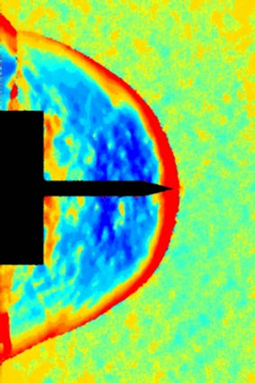 (b)
(b)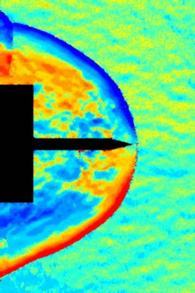 (c)
(c)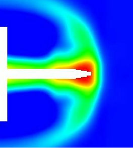 (d)
(d)
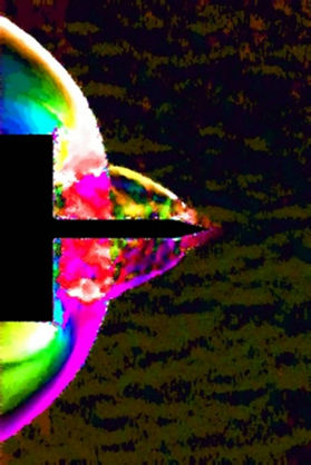
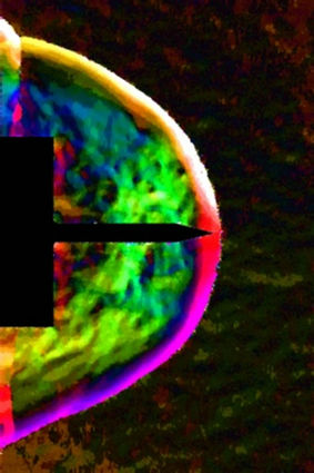
Figure 8. Flow visualization around the spike at t = 222 μs. (a) Pseudo color schlieren for the displacements; (b) Horizontal displacements; (c) Vertical displacements; (d) Reconstructed density on a midplane.
 (a)
(a)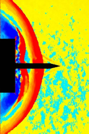 (b)
(b)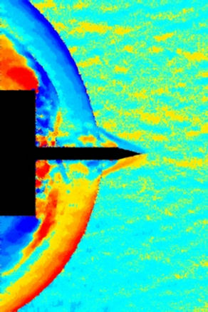 (c)
(c)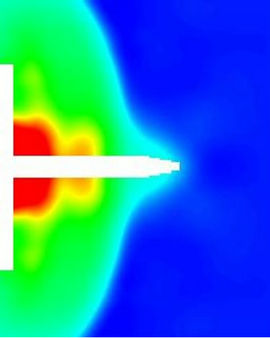 (d)
(d)
Figure 9. Flow visualization around the spike at t = 296 μs. (a) Pseudo color schlieren for the displacements; (b) Horizontal displacements; (c) Vertical displacements; (d) Reconstructed density on a midplane.
 (a)
(a)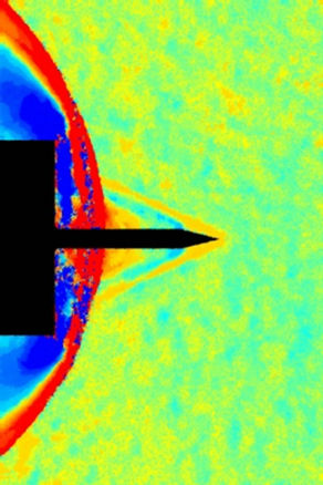 (b)
(b)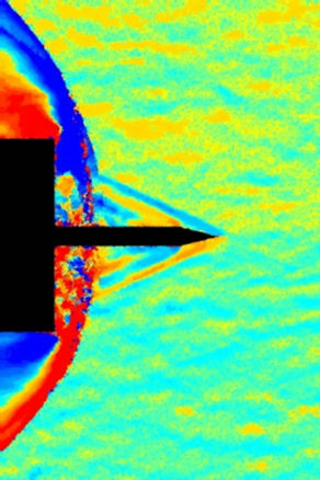 (c)
(c)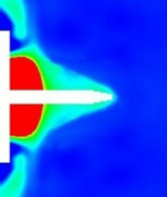 (d)
(d)
Figure 10. Flow visualization around the spike at t = 370 μs. (a) Pseudo color schlieren for the displacements; (b) Horizontal displacements; (c) Vertical displacements; (d) Reconstructed density on a midplane.
tion are recorded with a high-resolution camera (Canon EOS 1 Ds Mark II) with a normal lens (f = 50 mm). The CMOS sensor of the camera has a resolution of 4992 × 3328 pixels. The background is illuminated by a flashlamp for a duration of 2.5 μs [25]. In order to increase the depth of field, all pictures are taken with the smallest aperture, while the cameras are focused on the artificial background.
4. Reconstruction of the Flow Field
The Algebraic Reconstruction Technique (ART) is an iterative reconstruction method. The unknown density field is discretized and for each voxel (“volumetric pixel”) the density gradients and finally the density has to be determined. In order to solve this array of unknowns the Equations (2) have to be set for the measured displacement vectors for each projection as a function of the den-
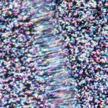
Figure 11. Blurred image of the dot pattern due to strong density gradients in the flow (detail of Figure 3).
 (a)
(a)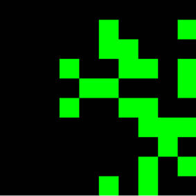 (b)
(b)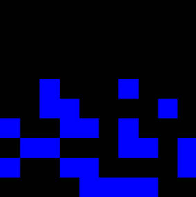 (c)
(c)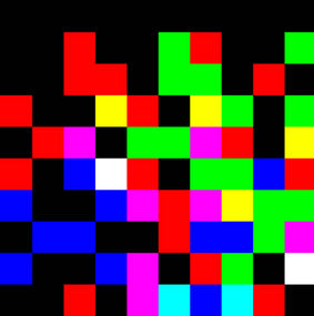 (d)
(d)
Figure 12. Structure of a background for regions with high density gradients. (a) Distribution of the red dots; (b) Distribution of the green dots due to the shift of the red dot pattern in horizontal direction; (c) Distribution of the blue dots due to the shift of the red dot pattern in vertical direction; (d) Superpostion of all dot patterns.
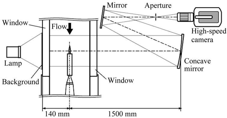
Figure 13. Telecentric optical setup proposed by Ota et al. [24].
sity gradient at the voxel [13]. ART is much simpler than the Filtered Back Projection method (FBP), which is based on the Fourier transform [14]. For FBP a large number of projections are required for a good reconstruction. In addition, the flow field around a model has to be reconstructed from incomplete projection data due to the obstruction caused by the model. As described by Sourgen et al. [15], obstructed parts have to be filtered or interpolated for the FBP algorithm in order to avoid the numerical artifacts. A comparison between the FBP and ART reconstruction algorithms based on the same LICT (Laser Interferometric Computed Tomography) measurements can be found in Ota et al. [13].
In this paper the new approach to the three-dimensional ART reconstruction and integration process is developed in order to achieve the three-dimensional density distribution based on CBOS data. In previous investigations [13], the Poisson’s equation was used to determine the density distribution [13,14].
The iteration process of the new approach can be described as follows:
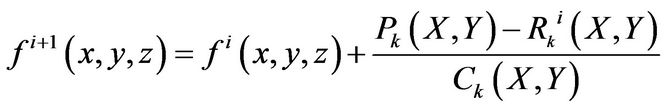 (3)
(3)
where fi denotes the density gradient distribution at step i, Pk stands for the measured displacement vectors in the projection map k, Rki denotes the estimated displacement vectors from the density distribution f i at step i, Ck the number of voxels along a projection line; x, y, z represent the coordinates in the density field and X and Y indicate the position in the projection map k.
In order to start the iteration process, the initial distribution of the density gradients f0 (x, y, z) is set to zero. Then the displacement vectors are estimated according to Equation (2) for the first projection . Taking into account the measurements for the first projection, a new estimation for the density gradients can be calculated. This process is applied to all projections. The three-dimensional distribution of the density is obtained by a linear integration of the density gradients in the x, y and z directions respectively. At least 30 iterations over the total number of projections are necessary in order to get a converged solution. In order to estimate the accuracy of the reconstruction, several theoretical test cases as well as a comparison with a reconstruction based on the Abel transformation has been carried out [13,14,22]. Earlier studies by Ota et al. [14] showed that good reconstruction data can be obtained from 36 projection angles ranging from 0˚ to 175˚ with intervals of 5˚. This configuration leads to an underestimation for the density of about 7% even in regions with high gradients.
In this case, assuming that the flow is axially symmetrical, every projection perpendicular to the symmetry axis should look the same. Earlier studies by Ota et al. [14] showed that good reconstruction data can be obtained from 36 projection angles ranging from 0˚ to 175˚ with intervals of 5˚. This configuration leads to an underestimation for the density of about 7% even in regions with high gradients. For the reconstruction of the flow field 152 ´ 240 ´ 240 voxels are used, which corresponds to a
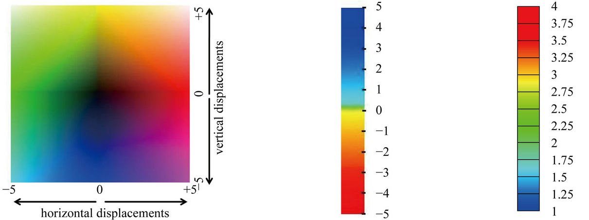 (a) (b) (c)
Figure 14. Legends for the Figures 5-10. (a) Color scale for the pseudo schlieren image [pixel]; (b) Color scale for the displacement values [pixel]; (c) Normalized density ρ/ρ∞.
distance between the voxels of 0.2 mm.
5. Experimental Results
In Figures 5 to 10 the displacements of the flow around the spike are represented at different instants of time. The size of the interrogation window for the CBOS evaluation is 10 ´ 10 pixels for all images, with an overlapping of 80%. In column a) pseudo color schlieren images are shown. These images show the vertical and horizontal displacements at the same time. In Columns b) and c) the horizontal and vertical displacements are shown respectively. In Column d) the results from the density reconstruction are shown. The color scales for the Figures 5 to 10 can be found in Figure 14.
Figure 5(a) shows the initially expected steady flow pattern, which is known from longer spikes (l/D > 1.2): a shock from the tip, followed by an expansion fan at the end of the conical tip. Furthermore a normal shock at the front of the cylinder can be seen. The isosurface for the density in Figure 5(d) shows the conical shock from the spike tip. The radial distribution of the density in front of the cylinder (Figure 6(d)) indicates the cushion-like high density zone in front of the cylinder. Nevertheless, the density gradients over the conical shock, which is very small compared to the grid size, are already underestimated with the CBOS measurement. Therefore the reconstructed density behind the shock is 12% lower than the value derived from theoretical considerations for conical shocks. In contrast the high density in front of the cylinder is well predicted.
Figure 6 reveals that disturbances propagate upstream, causing the conical shock to bulge. These disturbances travel up to the tip of the spike and lead to a detachment of the shock in front of the spike (Figure 7). This shock pattern looks like an established bow shock around a blunt body (Figure 8). The determined density due to the reconstruction behind the normal shock is 10% below the theoretical value for a normal shock at a Mach number 3.
The density distribution of the reconstructed image of Figure 8(d) clearly shows that the detached bow shock causes a considerably stronger compression than the initial conical shock pattern. As a result, the detached shock in front of the cylinder, which is still clearly visible in Figure 7, disintegrates.
As already mentioned in [18], the air around the spike does not withstand the pressure of the incoming flow as the wider shock layer allows the high-pressure gas to escape around the shoulder of the cylinder. The flow then pushes the bow shock back towards the model and a conical flow pattern is formed once again at the tip of the spike (Figure 9). As this conical region grows, a new shock appears in front of the cylinder (Figure 10). Approximately 480 μs later the flow field is nearly identical to the one observed in Figure 5. The main frequency of the fluctuation, measured with pressure tabs, is 2.063 kHz.
6. Conclusions
The Background Oriented Schlieren technique is a promising tool for the three-dimensional analysis of a flow with density gradients. In comparison with traditional methods, like the schlieren method, differential interferometry, etc., the BOS method is acknowledged for its simple optical setup and easy handling. In the case of the CBOS technique and due to the colored background, eight different dot patterns can be recorded simultaneously with one camera. Therefore, for every measurement eight independent correlations can be performed. The problems occurring in regions with strong shocks can be overcome by correlation between the different colored dot patterns.
The accuracy and the spatial resolution of the CBOS technique allow us to obtain a reliable reconstruction of the nearly axial symmetrical density field of unsteady flows. Especially for complex flows around a spiketipped model the distribution of the density helps considerably to understand the flow phenomena.
REFERENCES
- G. S. Settles, “Schlieren and Shadowgraph Techniques,” Springer, Berlin, Heidelberg and New York, 2001, pp. 1- 24.
- S. Debrus, M. Francon., C. P. Grover, M. May and M. L. Robin, “Ground Glass Differential Interferometer,” Applied Optics, Vol. 11, No. 4, 1972, pp. 853-857. doi:10.1364/AO.11.000853
- U. Köpf, “Application of Speckling for Measuring the Deflection of Laser Light by Phase Objects,” Optics Communications, Vol. 5, No. 5, 1972, pp. 347-350. doi:10.1016/0030-4018(72)90030-2
- U. Wernekink and W. Merzkirch, “Speckle Photography of Spatially Extended Refractive-Index Fields,” Applied Optics, Vol. 26, No. 1, 1987, pp. 31-32.
- R. Niessen, H. J. Schäfer and W. Merzkirch, “Measurement of Length Scales in the Turbulent Wake behind a Cylindrical Body at Supersonic Flow Velocities,” IUTAM Symposium on Eddy Structure Identification in Free Turbulent Shear Flows, Poitiers, September 1992, pp. 132- 138.
- G. E. A. Meier, “Hintergrund-Schlierenverfahren,” German Patent Office, No. 19942856.5, 1999.
- M. Raffel, H. Richard and G. E. A. Meier, “On the Applicability of Background Oriented Optical Tomography,” Experiments in Fluids, Vol. 28, No. 5, 2000, pp. 447-481.
- H. Richard and M. Raffel, “Principle and Applications of the Background Oriented Schlieren (BOS) Method,” Measurement Science and Technology, Vol. 12, No. 9, 2001, pp. 1576-1585. doi:10.1088/0957-0233/12/9/325
- L. Venkatakrishnan and G. E. A. Meier, “Density Measurements Using the Background Oriented Schlieren Technique,” Experiments in Fluids, Vol. 37, No. 2, 2004, pp. 237-247. doi:10.1007/s00348-004-0807-1
- L. Venkatakrishnan and P. Suriyanarayanan, “Density Field of Supersonic Separated Flow Past an Afterbody Nozzle Using Tomographic Reconstruction of BOS Data,” Experiments in Fluids, Vol. 47, No. 3, 2009, pp. 463-473. doi:10.1007/s00348-009-0676-8
- F. Sourgen, F. Leopold and D. Klatt, “Reconstruction of the Density Field Using the Colored Background Oriented Schlieren Technique,” Optics in Lasers and Engineering, Vol. 50, No. 1, 2012, pp. 29-38. doi:10.1016/j.optlaseng.2011.07.012
- A. C. Kak and M. Slaney, “Principle of Computerized Tomographic Imaging,” IEEE Press, New York, 1988.
- M. Ota, K. Hamada, H. Kato and K. Maeno, “ComputedTomographic Density Measurement of Supersonic Flow Field by Colored-Grid Background Oriented Schlieren (CGBOS) Technique,” Measurement Science and Technology, Vol. 22, No. 10, 2011, Article ID: 104011. doi:10.1088/0957-0233/22/10/104011
- M. Ota, H. Kato and K. Maeno, “Three-Dimensional Density Measurement of Supersonic and Axisymmetric Flow Field by Colored Grid Background Oriented Schlieren (CGBOS) Technique,” International Journal of Aerospace Innovations, Vol. 4, No. 1-2, 2012, pp. 1-11. doi:10.1260/1757-2258.4.1-2.1
- L. E. Ericsson, “Flow Pulsations on Concave Conic Forebodies,” Journal of Aircraft, Vol. 15, No. 5, 1978, pp. 287-292.
- A. G. Panaras, “Pulsating Flows about Axisymmetric Concave Bodies,” AIAA Journal, Vol. 19, No. 6, 1981, pp. 804-806. doi:10.2514/3.7816
- W. Calarese and W. L. Hankey, “Modes of Shock-Wave Oscillations on Spike-Tipped Bodies,” AIAA Journal, Vol. 23, No. 2, 1985, pp. 185-192. doi:10.2514/3.8893
- K. Hiraki, H. Kleine, H. Maruyama, T. Hayashid and K. Kitamura, “Flow Instability Induced by Spiked Bodies,” Proceedings of the SPIE 7126, 28th International Congress on High-Speed Imaging and Photonics, 71260K, Canberra, 10 February 2009. doi:10.1117/12.823751
- F. Leopold, J. Simon, D. Gruppi and H. J. Schäfer, “Recent Improvements of the Background Oriented Schlieren Technique (BOS) by Using a Colored Background,” 12th International Symposium on Flow Visualization, Göttingen, 10-14 September 2006, 10 p.
- J. Westerweel, “Digital Particle Image Velocimetry, Theory and Application,” Delft University Press, Delft, 1993.
- F. Klinge and M. L. Riethmuller, “Local Density Information Obtained by Means of the Background Oriented Schlieren (BOS) Method,” 11th International Symposium on Application of Laser Techniques to Fluid Mechanics, Lisbon, July 2002, Paper No. 3-2.
- F. Sourgen, J. Haertig and C. Rey, “Comparison between Background Oriented Schlieren Measurements (BOS) and Numerical Simulations,” 24th AIAA Aerodynamic Measurements Technology and Ground Testing Conference, Portland, 2004, Paper No. 2004. doi:10.2514/6.2004-2602
- K. Kindler, E. Goldhahn, F. Leopold and M. Raffel, “Recent Developments in Background Oriented Schlieren Methods for Rotor Blade Tip Vortex Measurements,” Experiments in Fluids, Vol. 43, No. 2-3, 2007, pp. 233- 240. doi:10.1007/s00348-007-0328-9
- M. Ota, H. Kato and K. Maeno, “Improvements of Spatial Resolution of Colored-Grid Background Oriented Schlieren (CGBOS) by Introducing Telecentric Optical System,” Proceedings of the 15th International Symposium on Flow Visualization, Minsk, July 2012, pp. 1-10.
- F. Leopold, “The Application of the Colored Background Oriented Schlieren Technique (CBOS) to Free-Flight and In-Flight Measurements,” Journal of Flow Visualization and Image Processing, Vol. 16, No. 4, 2009, pp. 279-293. doi:10.1615/JFlowVisImageProc.v16.i4.10