Advances in Remote Sensing
Vol.2 No.1(2013), Article ID:28972,6 pages DOI:10.4236/ars.2013.21004
Trend Analysis of Small Scale Commercial Sugarcane Production in Post Resettlement Areas of Mkwasine Zimbabwe, Using Hyper-Temporal Satellite Imagery
1Africa Institute of South Africa, Science and Technology Programme, Pretoria, South Africa 2Council for Scientific and Industrial Research (CSIR), Earth Observation Research Group, Natural Resource and Environment Unit, Pretoria, South Africa
3Department of Water Affairs, Hydrogeology Section, Pretoria, South Africa
Email: SMutanga@yahoo.com
Received December 10, 2012; revised January 16, 2013; accepted January 24, 2013
Keywords: Trend Analysis; Spot Vegetation; NDVI and Sugarcane
ABSTRACT
This study used normalized difference vegetation index (NDVI) derived from Spot Vegetation images as a proxy for sugarcane growth and production model. Time series analysis was undertaken using the moving average computed in R Programming language to monitor sugarcane production after the inception of land reform in the Mkwasine Estate of Zimbabwe. Overall the findings showed a declining trend with a few years of improved production over the 11 year period under investigation. To attest the possible explanations for the observed trend the study related NDVI data with climate variables and considered non climate factors such as land tenure. The predicted yield estimates over the years correlated very well with rainfall. The study therefore envisaged that hyper-temporal satellite imagery can be used to monitor sugarcane production and enhance decision making for future policy direction.
1. Introduction
As the Zimbabwean fast track land resettlement programme (FTLRP) of 2000 came into being, a substantial amount of land under sugarcane production was transferred to black growers, particularly in the Mkwasine Estate of the eastern lowveld. In order to optimize sugarcane quality, maximize its production, revenue to farmers, millers and the nation at large and aid the future policy direction [1] one of the key exercises is to monitor and evaluate the production trends. This work incorporated a sugarcane growth model based on the normalized difference vegetation index (NDVI) [2] from Spot Vegetation, to monitor the production trend after the inception of the land reform.
Sugarcane is a perennial crop of the Saccharum genus that is grown in the warm tropics and sub tropics [3] mainly for sugar and increasingly for biofuel production [4]. Sugarcane is a C4 plant that sinks carbon therefore helps in offsetting climate change. In [5], Zimbabwe has invested $600 m in a plant with a capacity of producing 500 million liters of ethanol at a massive cost of 50,000 ha of land for sugarcane production.
Advances in remote sensing technology and theory have expanded opportunities to characterize the inter-annual dynamics of natural and managed vegetation communities [6]. Approaches to the analysis of time series remotely sensed imagery have varied considerably, from standardized principal component analysis [7], to textural analysis [8], to the development of phonological metrics [9, 10], to the application of fourier analysis, also referred to as harmonic analysis which decomposes a time-dependent periodic phenomenon into a series of sinusoidal functions [11]. While harmonic analysis have proven to be a valuable technique, the interpretation of its results requires a consideration of several key components among which includes: a) each wave is defined by a unique amplitude and phase angle; b) the additive or zero term is the arithmetic mean of the variable over the time series; c) high amplitude values for a given term indicate a high level of variation in temporal variable time series; d) phase indicates the time of year at which the peak value for a term occurs [12]. This, study analyzed the Spot Vegetation—NDVI Time Series for sugarcane using a moving average technique, which is easy to implement and well embedded within the open source R programming software.
2. Methodology
2.1. Study Area
This study was conducted at Mkwasine Estate located in the lowveld region of Zimbabwe. This region is characterized by low and erratic summer precipitation of less than 450 mm per annum and high temperatures of around 35˚C. Sugarcane is thus grown under irrigation as the conditions are conducive for the growth of the crop within a 12-month cycle. Out of the 45,000 hectares of sugarcane plantations, 9000 ha are managed by 840 small to medium scale out growers under the Commercial Sugarcane Farmers Association (CSFA) and the Zimbabwe Sugarcane Farmers Association (ZSFA) [13]. Figure 1 shows the geographic location of the study area, which has a historical trend of contested land resource, following the fast track resettlement program of the year 2000.
2.2. Sampling, Data Collection and Analysis
A ground truthing exercise was carried out to collect sugarcane production data in the field using stratified random sampling based on whether the farmers produced sugarcane or other crops. A sample of twenty sugarcane plots was selected randomly within the forty identified each averaging an area between 12 and 40 hectares. Coordinates for each plot were taken. All the plots comprised of ratoon crops which are normally harvested at about 12 month interval for 4 years or more, before the crop is renewed. Actual yield levels were obtained from Mkwasine milling plant, where the resettled farmers sell their sugarcane output.
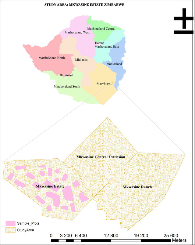
Figure 1. Location of study areas.
Hyper temporal satellite imagery in form of composite 10 days decadal NDVI images (S10 products) at 1 km × 1 km resolution from April 1998 to December 2009 for the study were extracted from Spot-4 Vegetation.
The Spot (Systeme Pour l’ Observation de la Terre) vegetation system have a spatial resolution of 1.15 km at nadir and a swath width of 2250 kilometers that can cover almost all the globe’s landmasses while orbiting 14 times a day [14]. It comprises of bands 2 (red; 0.61 - 0.68 µm) and 3 (near IR; 0.78 - 0.89 µm) which are the main wavelength bands for deriving the NDVI. The NDVI indicates chlorophyll activity and was calculated from (band 3 − band 2)/(band 3 + band 2); then index was converted to a digital number (DN value) in the 0 - 255 data range using: DN = (NDVI + 0.1)/0.004. The index was converted to 0 - 255 format so that it can be data handy with image classification software [15]. The downloded NDVI images were geo-referenced and declouded. Declouded means: using by image and pixel the supplied quality record, only pixels with a “good” radiometric quality for bands 2 (red; 0.61 - 0.68 µm) and 3 (near IR; 0.78 - 0.89 µm), and not having “shadow” “cloud” or “uncertain”, but “clear” as general quality, were kept (removed pixels were labeled as “missing”) [16].
The randomly selected sugarcane plots were used to extract the NDVI on the SPOT Images. Zonal Statistics was applied to get the hyper temporal mean and maximum NDVI for all the sample plots. Considering vegetation phenol-phases are sensitive to certain environmental controls [17-19] the study compared maximum and mean NDVI per plot with climate variables such as rainfall. These variables have been a proxy to help explain the yield estimation trend [20]. Figure 2 shows the simplified methodological Approach for the study.
2.3. Time Series Analysis
The time series analysis was done in the moving average as implemented in an open source software called R-programming language [21]. Firstly the time series NDVI was translated into the time series objects using the “ts” function [22], and the specified frequency was 12 months, and the start of the time series data was 1998. Secondly, components such as trend, seasonal and random or irregular were extracted from the time series data using the “Decompose” function which applies the moving average [21]. The Decompose approach utilizes the additive and multiplicative seasonal components [21] illustrated in Equations (1) and (2).
The additive model used is:
 (1)
(1)
The multiplicative model used is:
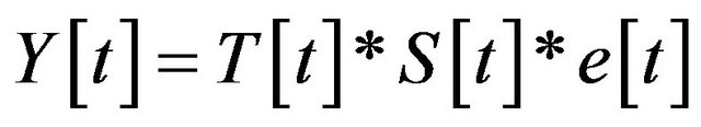 (2)
(2)
where t is time, T is trend, S is seasonal and e is the error or irregular component.

Figure 2. Simplified Schema of the methodological Approach.
The decompose function firstly determines the trend component using a moving average i.e. a symmetric window with equal weights, and removes it from the time series. Secondly, the seasonal figure is computed by averaging, for each time unit, over all periods. Thirdly, the error component is determined by removing trend and seasonal figure (recycled as needed) from the originnal time series. More details about this approach can be found in [21].
To test the general trends statistically, the autocorrelation were computed using the auto correlation function estimation (acf) and partial autocorrelation (pacf) [23]. The estimates acf and pacf are based on data or sample covariance. The lag 0 autocorrelation is always fixed at 1 by convention, since it is a correlation of the same initial values. The profile of NDVI indicates a similar pattern for all the plots hence the mean and maximum profile was used to undertake the trend analysis.
3. Results & Discussion
The time series NDVI, a proxy for estimated sugarcane yield from 1998 to 2009 is statistically depicted by the trend components (trend, seasonal and random) and the computed autocorrelation shown in Figures 3 and 4 respectively. The data profile on Figure 3 shows the variability in sugarcane production being characterized by an irregular pattern over the period 1998-2005, while the later years are generally uniform and cyclical in nature.
The trend profile on Figure 3 shows a general trend of decline in NDVI from the year 1999, with a slight increase in 2001, and a significant drop in 2002. From the year 2003 the NDVI increased until it reached its peak in
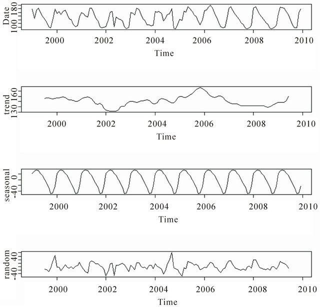
Figure 3. Trend components: Data, the decomposed time series (trend, seasonal and irregular/random components).
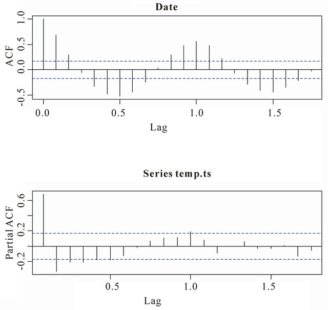
Figure 4. Autocorrelation and the partial autocorrelation estimation derived from the time series data.
2006 and then decreased up to 2009. The declining and increasing trends have been qualified by the estimated autocorrelation and partial autocorrelation shown in Figure 4. Overall the findings showed a declining trend with a few years of improved production over the 11 year period under investigation.
Several explanations for the changes in the NDVI for the study period exist. The main reason for the probable significant fluctuations is the land reform that was carried out in the area and country at large from the beginning of the year 2000. The land reform was characterized by major changes in the land tenure from mainly commercial farms and estates to a mixture of the commercial farms, estates and small scale sugarcane farmers.
Often some of the resettled small scale farmers lacked the experience in sugarcane production, the necessary inputs and chemicals such that the yields declined as supported by the NDVI trend. Reduced investor confidence in the sugarcane industry following the decade long political instability in Zimbabwe might have contributed to the decline in production. Complemented to this has been the country’s economic recession which accentuated small scale famers’ lack of capacity to procure irrigation equipment, tractors, and paying for other farming inputs.
Results of this study were consistent with Zvoutete’s [13], findings that there has been a marked decrease in the sugarcane output since the inception of the land reform in Zimbabwe. In his study from the smut disease perspective (a sugarcane disease), its prevalence after the land reform has been recorded as the highest levels ever in the country with no measures of controlling the disease resulting in up to a significant 15% loss in the sugarcane output.

Figure 5. Relationship between maximum NDVI and growing seasonal Rainfall.
Climate variables could possibly have influenced the behavior of the NDVI profiles. The relationship between mean, maximum NDVI and rainfall was positive with an R2 of 0.65 as indicated in Figure 5. This study thus concur with the previous analysis by Ding et al. [24] which found out that the correlation between annual effective rainfall and annual maximum NDVI was similar to the growing seasonal rainfall. In addition Wu et al. [25], found out that warm-humid trend influenced by climatic variability positively affects vegetation growth which in this case is the effect on sugarcane crop. Therefore climate extremes can help explain the trends. The poor rains received in the 2008 to 2009 agricultural season might have contributed to the declining trend.
4. Conclusion
Remotely sensed data in particular hyper-temporal satellite imagery (Spot Vegetation), can be used satisfactorily to estimate the sugarcane production trends over the years. The main findings of this study showed a declining trend with a few years of improved production over the 11 year period under investigation. The study identified a wide range of factors that could possibly help explain the general production trend among which includes land reform, human capital, economic factors, and climate variables. However this study recommends a comparative analysis of the trend in production before and after the land reform in order to ascertain the net benefit of the programme.
5. Acknowledgements
This research is sponsored by the Africa Institute of South Africa, a science council under the Department of Science and Technology mandated to produce knowledge aimed at informing sustainable political and socioeconomic development in Africa.
REFERENCES
- W. G. M. Bastiaanssen and S. Ali, “A New Crop Yield Forecusting Model Based on Satellite Measurements Applied across the Inuds Basin, Pakistan,” Agriculture, Ecosystem and Environment, Vol. 94, No. 3, 2003, pp. 321- 340. doi:10.1016/S0167-8809(02)00034-8
- L. A. S. Romani, R. R. V. Goncalves, J. R. Zullo, J. R. Traina and A. J. M. Traina, “New DTW-Based Method to Similarity Search in Sugar Cane Regions Represented by Climate and Remote Sensing Time Series,” International Geoscience and Remote Sensing Symposium, Hawaii, 25- 30 July 2010, pp. 355-358.
- B. Amigun, J. Musango and W. Stafford, “Biofuels and Sustainability in Africa,” Renewable and Sustainable Energy Reviews, Vol. 15, No. 2, 2011, pp. 1360-1372.
- USDA, “Zimbabwe Sugar Annual Global Agricultural Information Network,” 2010.
- M. E. Jakubauskas, D. R. Legates and J. H. Kastens, “Harmonic Analysis of Time-Series AVHRR NDVI Data,” Photogrammetric Engineering & Remote Sensing, Vol. 67, No. 4, 2001, pp. 461-470.
- J. R. Eastman and M. Fulk, “Long Sequence Time Series Evaluation Using Standardized Principal Components,” Photogrammetric Engineering & Remote Sensing, Vol. 59, No. 8, 1993, pp. 1307-1312.
- J. Brims and M. D. Nellis, “Seasonal Variation of Heterogeneity in the Tall Grass Prairie: A Quantitative Measure Using Remote Sensing,” Photogrammetric Engineering & Remote Sensing, Vol. 57, No. 4, 1991, pp. 407-411.
- D. Lloyd, “A Phenological Classification of Terrestrial Vegetation Cover Using Shortwave Vegetation Index Imagery,” International Journal of Remote Sensing, Vol. 11, No. 12, 1990, pp. 2269-2279. doi:10.1080/01431169008955174
- S. A. Samson, “Two Indices to Characterize Temporal Patterns in the Spectral Response of Vegetation,” Photogrammetric Engineering Remote Sensing, Vol. 59, No. 4, 1993, pp. 511-517.
- B. Reed, J. Brown, D. VanderZee, T. Loveland, J. Merchant and D. O. Ohlen, “Measuring Penological Variability from Satellite Imagery,” Journal of Vegetation Science, Vol. 5, No. 5, 1994, pp. 703-714. doi:10.2307/3235884
- M. E. Jakubauskas, D. R. Legates and J. H. Kastens, “Harmonic Analysis of Time-Series AVHRR NDVI Data,” Photogrammetric Engineering & Remote Sensing, Vol. 67, No. 4, 2001, pp. 461-470.
- J. N. Rayner, “An Introduction to Spectral Analysis,” Pion Ltd., London, 1971.
- P. Zvoutete, “Fluctuations in the Levels of SMUT (Ustilago Scitaminea) in Response to Changes in Disease Management Strategies in the Zimbabwe Sugarcane Industry,” Proceedings of South Africa Sugar Technological Association, Vol. 81, 2008, pp. 381-387.
- F. Van Der Meer, K. S. Schimdt and W. Bakker, “New Environmental Remote Sensing Systems,” Taylor Francis, London, 2002.
- A. Murwira, “Scale Matter!! A New Approach to Quantify Spatial Heterogeneity for Predicting the Distribuiton of Wildlife,” International Institute for Geo-Information Science & Earth Observation (ITC), Enschede, 2003.
- A. K. Skidmore, A. G. Toxopeus, K. De Bie, F. Corsi, V. Venus, D. P. Omolo and J. Marquex, “Hepertological Species Mapping for the Meditteranean,” In: Skidmore, Ed., ISPRS Commission VII Mid Term Sysmposium—Remote Sensing from Pixel to Processes, ISPRS, Enschede, 2006, p. 7.
- H. Hanninen, “Effects of Climate Change on Trees from Cool and Temperate Regions: An Ecophysical Approach to Modelling of Bud Burst Phenology,” Canadian Journal of Botany, Vol. 73, No. 2, 1994, pp. 183-199. doi:10.1139/b95-022
- P. R. Kemp, “Phenologic Patterns of Chihuahuan Desert Plants in Relationship to Timing of Water Availability,” Journal of Ecology, Vol. 71, No. 2, 1983, pp. 427-436. doi:10.2307/2259725
- W. Larcher, “Physiological Plant Ecology,” Springer-Verlag Press, Berlin, 1995. doi:10.1007/978-3-642-87851-0
- J. P. Jenkins, B. H. Braswell, S. E. Frolking and J. D. Aber, “Detecting and Predicting Spatial and Inter-Annual Patterns of Temperate Forest Springtime Phenology in the Eastern US,” Geophysical Research Letters, Vol. 29, No. 24, 2001, pp. 541-544. doi:10.1029/2001GL014008
- M. Kendall and A. Stuart, “The Advanced Theory of Statistics,” Griffin, Vol. 3, 1983, pp. 410-414.
- R. A. Becker, J. M. Chambers and A. R. Wilks, “The New S Language,” Wadsworth & Brooks/Cole, Monterey, 1988.
- W. N. Venables and B. D. Ripley, “Modern Applied Statistics with S,” 4th Edition, Springer-Verlag, Berlin, Heidelberg, 2002. doi:10.1007/978-0-387-21706-2
- Ding, et al., “The Relationship between NDVI and Precipitation on the Tibetan Plateau,” Journal of Geographical Sciences, Vol. 17, No. 3, 2007, pp. 259-268. doi:10.1007/s11442-007-0259-7
- S. H. Wu, Y. H. Yin, D. Zheng, et al., “Climate Changes in the Tibetan Plateau during the Last Three Decades,” Acta Geographica Sinica, Vol. 60, No. 1, 2005, pp. 1-11.