Pharmacology & Pharmacy
Vol.3 No.2(2012), Article ID:18709,9 pages DOI:10.4236/pp.2012.32021
The Assessment of Non-Linear Effects in Clinical Research
![]()
European College Pharmaceutical Medicine Lyon France, c/o Albert Schweitzer Hospital, Dordrecht, Netherlands.
Email: *ajm.cleophas@wxs.nl, a.j.m.cleophas@asz.nl
Received January 8th, 2012; revised February 16th, 2012; accepted March 4th, 2012
Keywords: Non-Linear Effects; Clinical Research; Logit/Probit Transformation; Box Cox Transformation; ACE/AVAS Packages; Curvilinear Data; Spline Modeling; Loess Modeling
ABSTRACT
Background: Novel models for the assessment of non-linear data are being developed for the benefit of making better predictions from the data. Objective: To review traditional and modern models. Results, and Conclusions: 1) Logit and probit transformations are often successfully used to mimic a linear model. Logistic regression, Cox regression, Poisson regression, and Markow modeling are examples of logit transformation; 2) Either the xor y-axis or both of them can be logarithmically transformed. Also Box Cox transformation equations and ACE (alternating conditional expectations) or AVAS (additive and variance stabilization for regression) packages are simple empirical methods often successful for linearly remodeling of non-linear data; 3) Data that are sinusoidal, can, generally, be successfully modeled using polynomial regression or Fourier analysis; 4) For exponential patterns like plasma concentration time relationships exponential modeling with or without Laplace transformations is a possibility. Spline and Loess are computationally intensive modern methods, suitable for smoothing data patterns, if the data plot leaves you with no idea of the relationship between the yand x-values. There are no statistical tests to assess the goodness of fit of these methods, but it is always better than that of traditional models.
1. Introduction
Non-linear relationships like the smooth shapes of airplanes, boats, and motor cars were constructed from scale models using stretched thin wooden strips, otherwise called splines, producing smooth curves, assuming a minimum of strain in the materials used. With the advent of the computer it became possible to replace it with statistical modeling for the purpose: already in 1964 it was introduced by Boeing [1] and General Motors [2]. Mechanical spline methods were replaced with their mathematical counterparts. A computer program was used to calculate the best fit line/curve, which is the line/curve with the shortest distance to the data. More complex models were required, and they were often laborious so that even modern computers had difficulty to process them. Software packages make use of iterations: 5 or more regression curves are estimated (“guesstimated”), and the one with the best fit is chosen. With large data samples the calculation time can be hours or days, and modern software will automatically proceed to use Monte Carlo calculations [3] in order to reduce the calculation times. Nowadays, many non-linear data patterns can be developed mathematically, and this paper reviews some of them.
2. Testing for Linearity
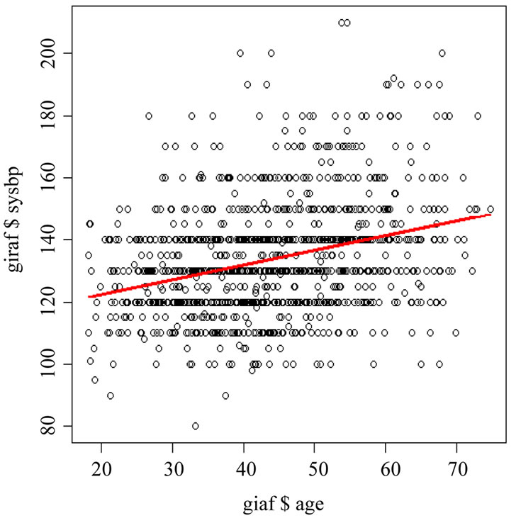
A first step with any data analysis is to assess the data pattern from a scatter plot (Figure 1).
A considerable scatter is common, and it may be difficult to find the best fit model. Prior knowledge about patterns to be expected is helpful.
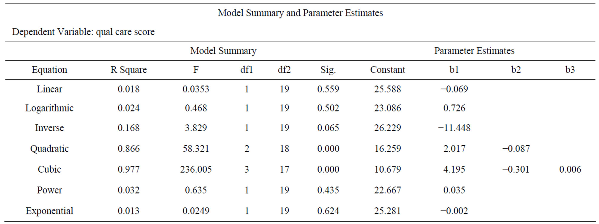
Sometimes, a better fit of the data is obtained by drawing y versus x instead of the reverse. Residuals of y versus x with or without adjustments for other x-values are helpful for finding a recognizable data pattern. Statistically, we test for linearity by adding a non-linear term of x to the model, particularly, x squared or square root x, etc. If the squared correlation coefficient r2 becomes larger by this action, then the pattern is, obviously, notlinear. Statistical software like the curvilinear regression option in SPSS [4] helps you identify the best fit model. Figure 2 and Table 1 give an example. The best fit models for the data given in the Figure 2 are the quadratic and cubic models.
In the next few sections various commonly used mathematical models are reviewed. The mathematical equations of these models are summarized in the appendix. They are helpful to make you understand the assumed nature of the relationships between the dependent and independent variables of the models used.
 (a)
(a)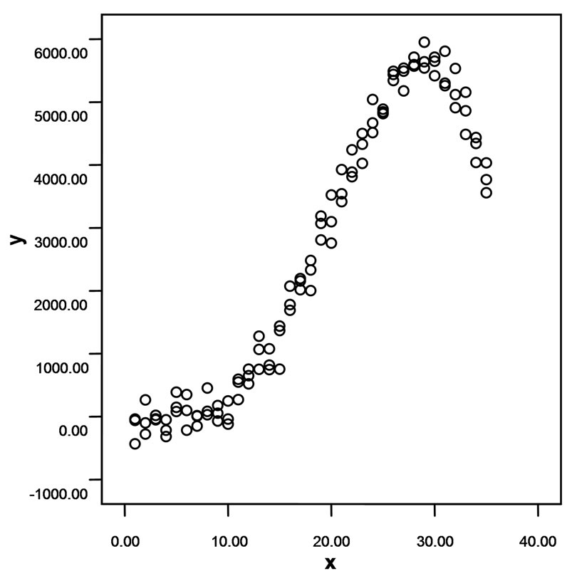 (b)
(b)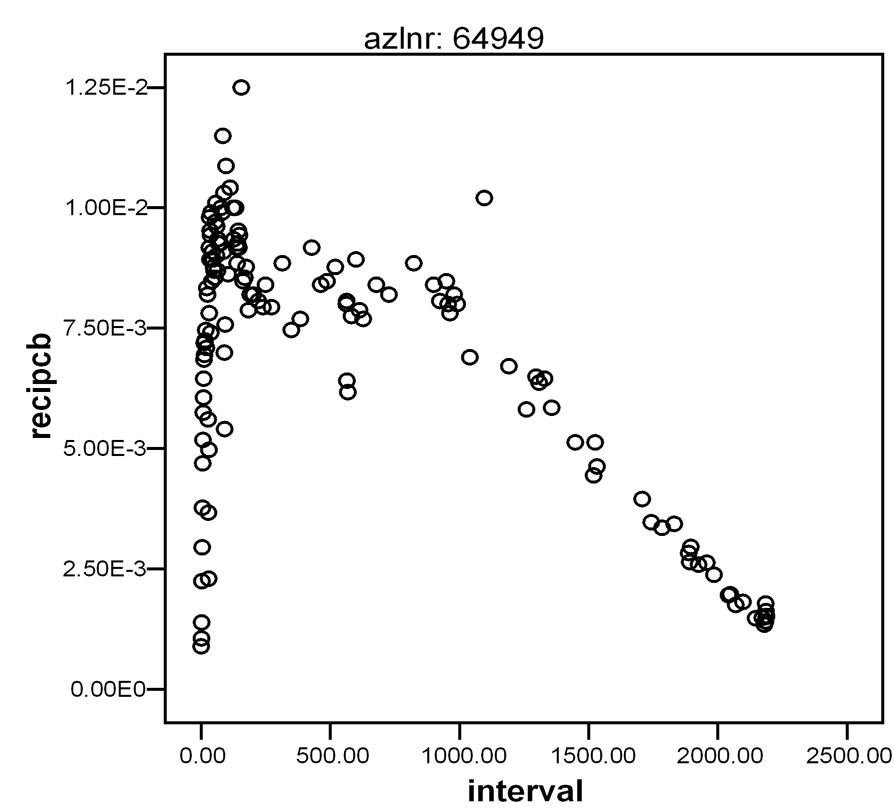 (c)
(c)
Figure 1. Examples of non-linear data sets: (a) Relationship between age and systolic blood pressure; (b) Effects of mental stress on fore arm vascular resistance; (c) Relationship between time after polychlorobiphenyl (PCB) exposure and PCB concentrations in lake fish.
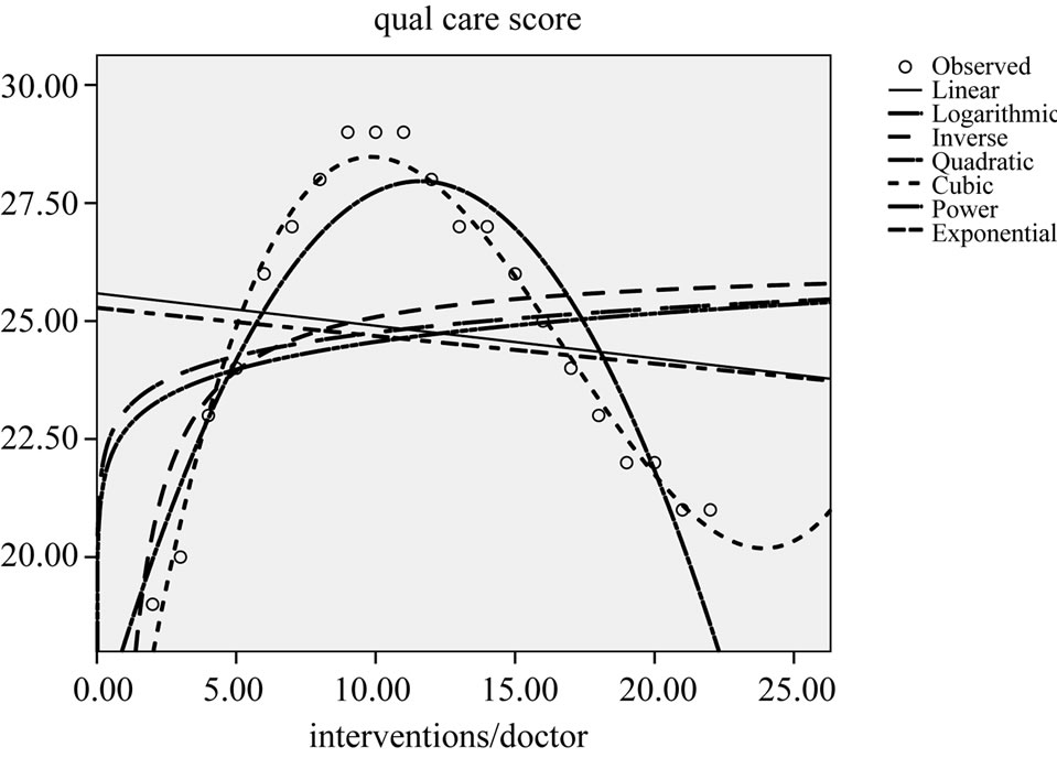
Figure 2. Standard models of regression analyses: the effect of quantity of care (numbers of daily interventions, like endoscopies or small operations, per doctor) is assessed against quality of care scores.
3. Logit and Probit Transformations
If linear regression produces a non-significant effect, then other regression functions can be chosen and may provide a better fit for your data. Following logit (=logistic) transformation a linear model is often produced. Logistic regression (odds ratio analysis), Cox regression (Kaplan-Meier curve analysis), Poisson regression (event rate analysis), Markov modeling (survival estimation) are examples. SPSS statistical software [4] covers most of these methods, e.g., in its module “Generalized linear methods”. There are examples of datasets where we have prior knowledge that they are linear after a known transformation (Figures 3 and 4). As a particular caveat we should add here that many examples can be given, but beware. Most models in biomedicine have considerable residual scatter around the estimated regression line. For example, if the model applied is the following (e = random variation)
yi = α eβx + ei,
then
ln(yi) ¹ ln(α) + βx + ei.
The smaller the ei term is, the better fit is provided by the model. Another problem with logistic regression is that sometimes after iteration (=computer program for finding the largest log likelihood ratio for fitting the data) the results do not converse, i.e., a best log likelihood ratio is not established. This is due to insufficient data size, inadequate data, or non-quadratic data patterns. An alternative for that purpose is probit modeling, which, generally, gives less iteration problems. The dependent variable of logistic regression (the log odds of responding) is closely related to log probit (probit is the z-value corresponding to its area under curve value of the normal distribution). It can be shown that log odds of responding =
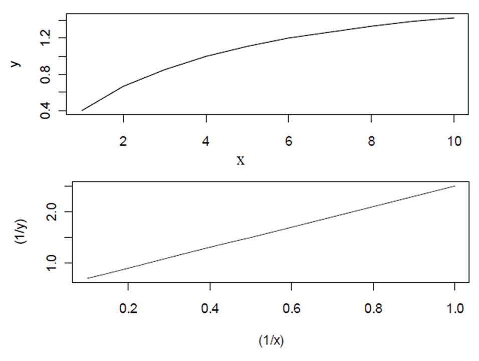
Figure 3. Example of non-linear relationship that is linear after log transformation (Michaelis-Menten relationship between sucrose concentration on x-axis and invertase reaction rate on y-axis).
logit ≈ (π/ )x probit. Probit analysis, although not available in SPSS, is in many software programs like, e.g., Stata [5].
4. “Trial and Error” Method, Box Cox Transformation, ACE/AVAS Packages
If logit or probit transformations do not work, then additional transformation techniques may be helpful. How do you find the best transformations? First, prior knowledge about the patterns to be expected is helpful. If this is not available, then the “trial and error” method can be recommended, particularly, logarithmically transforming either xor y-axis or both of them (Figure 5).
log(y) vs x, y vs log(x), log(y) vs log(x).
The above methods can be performed by hand (vs = versus). Box Cox transformation [6], additive regression using ACE [7] (alternating conditional expectations) and AVAS [7] (additive and variance stabilization for regression) packages are modern non-parametric methods, otherwise closely related to the “trial and error” method, can also be used for the purpose.
They are not in SPSS statistical software, but instead a free Box-Cox normality plot calculator is available on the Internet [8]. All of the methods in this section are largely empirical techniques to normalize non-normal data, that can, subsequently, be easily modeled, and they are available in virtually all modern software programs.
5. Sinusoidal Data
Clinical research is often involved in predicting an outcome from a predictor variable, and linear modeling is the commonest and simplest method for that purpose. The simplest except one is the quadratic relationship providing a symmetric curve, and the next simplest is the
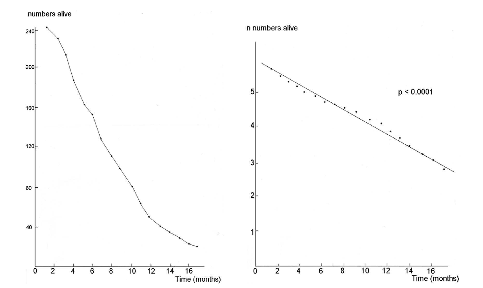
Figure 4. Another example of a non-linear relationship that is linear after logarithmic transformation (survival of 240 small cell carcinoma patients).
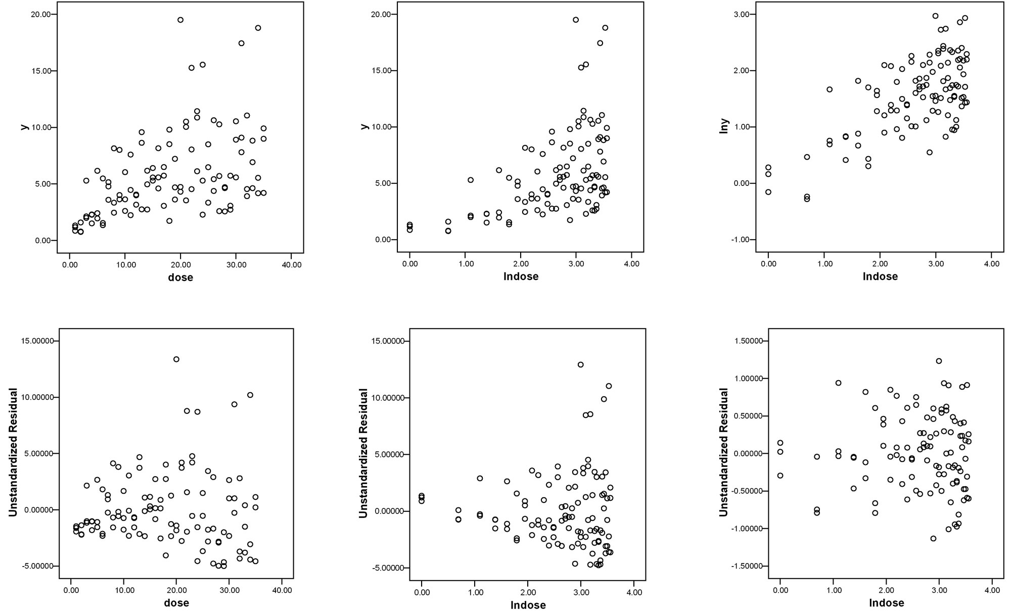
Figure 5. Trial and error methods used to find recognizable data patterns: relationship between isoproterenol dosages (on the x-axis) and relaxation of bronchial smooth muscle (on the y-axis).
cubic model providing a sinus-like curve.
The equations are
Linear model y = a + bx
Quadratic model y = a + bx2
Cubic model y = a + bx3.
The larger the regression coefficient b, the better the model fits the data. Instead of the terms linear, quadratic, and cubic the terms first order, second order, and third order polynomial are applied.
If the data plot looks, obviously, sinusoidal, then higher order polynomial regression and Fourier analysis could be adequate [9]. The equations are given in the appendix. Figure 6 gives an example of a polynomial model of the seventh order.
6. Exponential Modeling
For exponential-like patterns like plasma concentration time relationships exponential modeling is a possibility [10]. Also multiple exponential modeling has become possible with the help of Laplace transformations. The non-linear mixed effect exponential model (nonmen model) [11] for pharmacokinetic studies is an example (Figure 7). The data plot shows that the data spread is wide and, so, very accurate predictions can not be made in the given example. Nonetheless, the method is helpful to give an idea about some pharmacokinetic parameters like drug plasma half life and distribution volume.
7. Spline Modeling
If the above models do not adequately fit your data, you may use a method called spline modeling. It stems from the thin flexible wooden splines formerly used by shipbuilders and car designers to produce smooth shapes [1,2]. Spline modeling will be, particularly, suitable for smoothing data patterns, if the data plot leaves you with no idea of the relationship between the yand x-values.
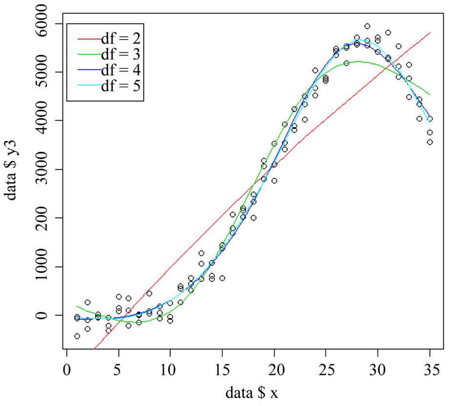
Figure 8 gives an example of non-linear dataset suitable for spline modeling. Technically, the method of local smoothing, categorizing the x-values is used. It means that, if you have no idea about the shape of the relation between the y-values and the x-values of a two dimensional data plot, you may try and divide the x-values into 4 or 5 categories, where θ-values are the cut-offs of categories of x-values otherwise called the knots of the spline model.
• cat. 1: min £ x < θ1
• cat. 2: θ1 £ x < θ2
• ...
• cat. k: θk−1 £ x < max.
Then, estimate y as the mean of all values within each category. Prerequisites and primary assumptions include
• the y-value is more or less constant within categories of the x-values
• categories should have a decent number of observations
• preferably, category boundaries should have some meaning.
A linear regression of the categories is possible, but the linear regression lines are not necessarily connected (Figure 9). Instead of linear regression lines a better fit for the data is provided by separate low-order polynomial
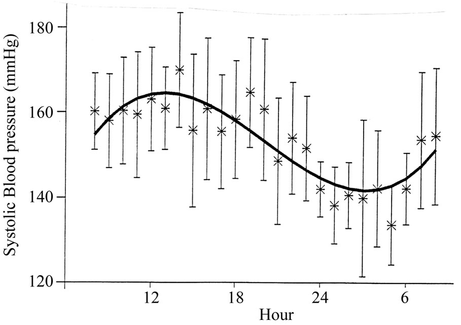
Figure 6. Example of a polynomial regression model of the seventh order to describe ambulatory blood pressure measurements.
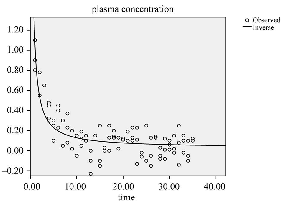
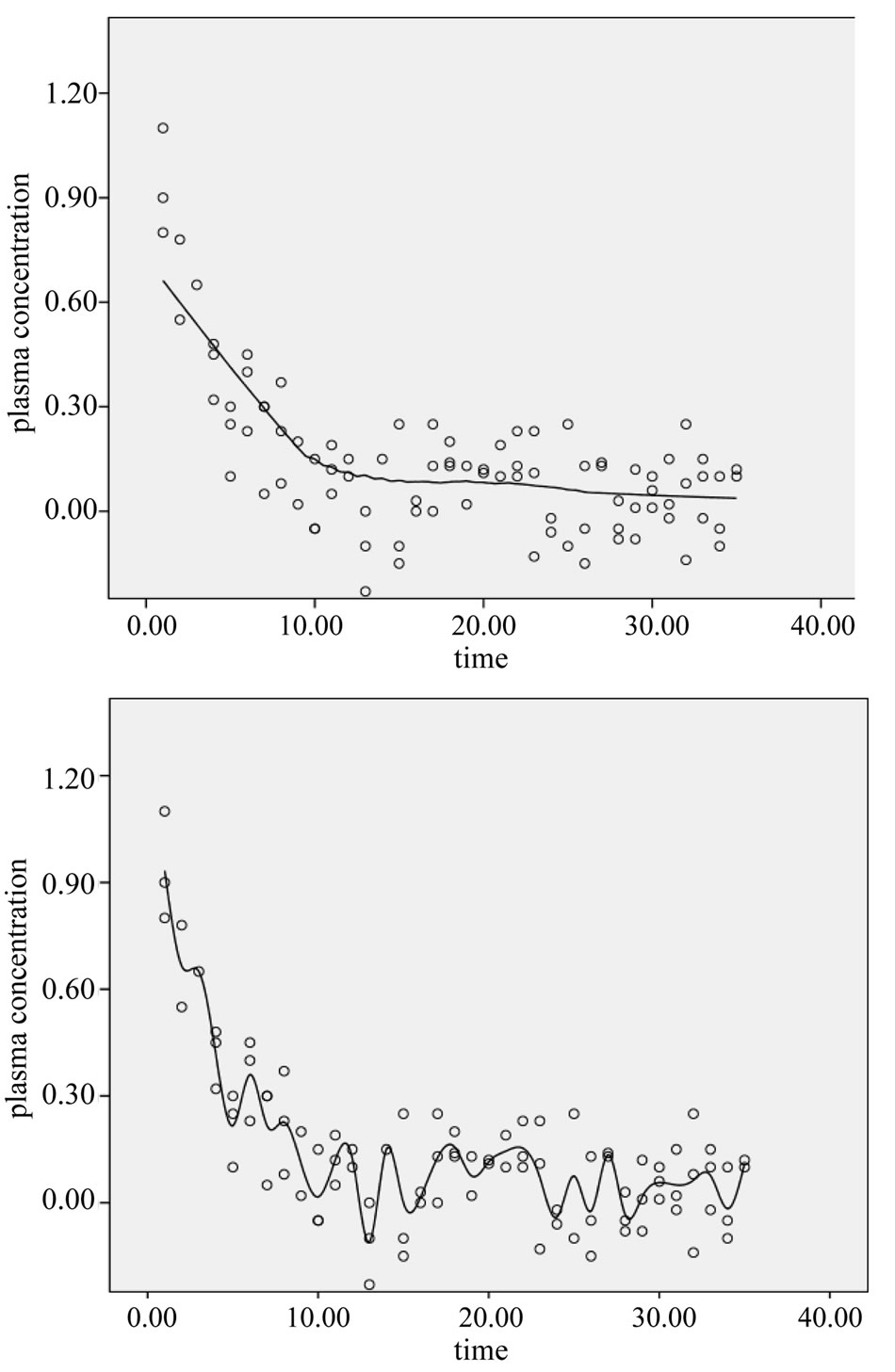
Figure 7. Example of exponential model to describe plasma concentration-time relationship of zoledronic acid.
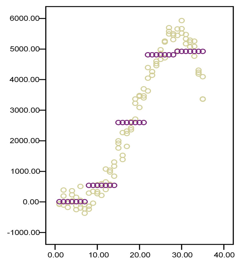
Figure 8. Example of a non-linear dataset suitable for spline modeling: effects of mental stress on fore arm vascular resistance.
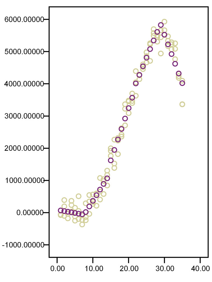
regression lines (Figure 10). for all of the intervals between two subsequent knots, where knots are x-values that connect one x-category with a subsequent one. Usually, cubic regression, otherwise called third order polynomial regression, is used. It has as simplest equation y = a + bx3 . Eventually, the separate lines are joined at the knots. Spline modeling, thus, cuts the data into 4 or 5 intervals and uses the best fit third order polynomial functions for each interval (Figure 11). In order to obtain a smooth spline curve the junctions between two subsequent functions must have
1) The same y value
2) The same slope
3) The same curvature.
All of these requirements are met if
1) The two subsequent functions are equal at the junction
2) Have the same first derivative at the junction
3) Have the same second derivative at the junction.
There is a lot of matrix algebra involved, but a computer program can do the calculations for you, and provide you with the best fit spline curve.
Even with knots as few as 2, cubic spline regression may provide an adequate fit for the data.
In computer graphics spline models are popular curves, because of their accuracy and capacity to fit complex data patterns. So far, they are not yet routinely used in clinical research for making predictions from response patterns, but this is a matter of time. Excel provides free cubic spline function software [11]. The spline model can be checked for its smoothness and fit using lambda-calcu-
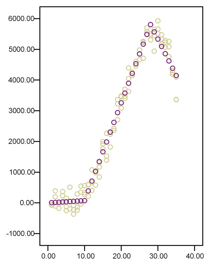
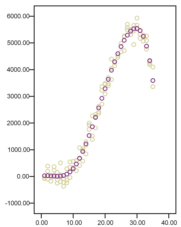
Figure 10. The first graph linear regression, the second graph cubic regression from the data from Figure 8.
lus [12], and generalized additive models [13,14]. Unfortunately, multidimensional smoothing using spline modeling is difficult. Instead you may perform separate procedures for each covariate. Two-dimensional spline modeling is available in SPSS:
Command: graphs chart builder basic elements choose axes y-x gallery scatter/dot ok double click in outcome graph to start chart editor elements interpolate properties mark: spline click: apply best fit spline model is in the outcome graph.
8. Loess Modeling
Maybe, the best fit for many types of non-linear data is offered by still another novel regression method called Loess (locally weighted scatter plot smoothing) [15]. This
computationally very intensive program calculates the best fit polynomials from subsets of your data set in order to eventually find out the best fit curve for the overall data set, and is related to Monte Carlo modeling. It does not work with knots, but, instead chooses the bets fit polynomial curve for each value, with outlier values given less weight. Loess modeling is available in SPSS:
Command: graphs chart builder basic elements choose axes y-x gallery scatter/dot ok double click in outcome graph to start chart editor elements fit line at total properties mark: Loess click: apply best fit Loess model is in the outcome graph.
Figure 12 compares the best fit Loess model with the best fit cubic spline model for describing a plasma concentration-time pattern. Both give a better fit for the data than does the traditional exponential modeling with 9 and 29 values in the Loess and spline lines compared to only 5 values in the exponential line of Figure 6. However, it is impossible to estimate plasma half life from Loess and spline. We have to admit that, with so much spread in the data like in the given example, the meaning of the calculated plasma half life is, of course, limited.
9. Discussion
Many tools are available for developing non-linear models for characterizing data sets and making predictions from them. Sometimes it is difficult to choose the degree of smoothness of such models: e.g., with polynomial regression the question is which order, and with spline modeling the questions are how many knots, which locations, which lambdas.
Another method is kernel frequency distribution modeling which unless histograms consists of multiple similarly sized Gaussian curves rather than multiple bins of
different length. In order to perform kernel modeling the bandwidth (span) of the Gaussian curves has to be selected which may be a difficult but important factor of the potential fit of a particular kernel method.
Irrespective of the smoothing method applied, there are some problems with smoothing: it may introduce bias, and, second, it may increase the variance in the data. The Akaike information criterion [17] (AIC) is a measure of the relative goodness of fit of a mathematical model for describing data patterns. It can be used to describe the tradeoff between bias and variance in model construction, and to assess the accuracy of the model used. However, the AIC, as it is a relative measure, will not be helpful to confirm a poor result, if all of the models fit the data equally poorly.
Disadvantages of computationally intensive methods like spline modeling and Loess modeling must be mentioned. They require fairly large, densely sampled data sets in order to produce good models. However, the analysis is straightforward. Another disadvantage is the fact that these methods do not produce simple regression functions that can be easily represented by mathematical equations. However, for making predictions from such models direct interpolations/extrapolations from the graphs can be made, and, given the mathematical refinement of these methods, these predictions should, generally, give excellent precision.
10. Conclusions
1) Logit and probit transformation can sometimes be used to mimic a linear model. Logistic regression, Cox regression, Poisson regression, and Markow modeling are examples of logit transformation.
2) Either the xor y-axis or both of them can be logarithmically transformed. Also Box Cox transformation equation and ace (alternating conditional expectations) or avas (additive and variance stabilization for regression) packages are simple empirical methods often successful for linearly remodeling non linear data.
3) Data that are, obviously, sinusoidal, can, generally, be successfully modeled using polynomial regression and Fourier analysis.
4) For exponential patterns like plasma concentration time relationships exponential modeling with or without Laplace transformations is a possibility.
5) Spline and Loess modeling are modern methods, particularly, suitable for smoothing data patterns, if the data plot leaves you with no idea of the relationship between the yand x-values. Loess tends to skip outlier data, while spine modeling rather tends to include them. So, if you are planning to investigate the outliers, then spline is your tool.
We have to add that traditional non-linear modeling produces p-values, and modern methods do not. However, given the poor fit of many traditional models, these pvalues do not mean too much. Also, it is reassuring to observe that both Loess and spline provide a better fit to non-linear data than does traditional modeling.
REFERENCES
- J. C. Ferguson, “Multi-Variable Curve Interpolation,” Journal of the Association for Computing Machinery, Vol. 11, No. 2, 1964, pp. 221-228. doi:10.1145/321217.321225
- F. Birkhof and R. De Boor, “Piecewise Polynomial Interpretation and Approximation,” Proceedings of General Motors Symposium of 1964, Elsevier Publishing Co., New York, pp. 164-190.
- T. J. Cleophas and A. H. Zwinderman, “Monte Carlo methods,” 4th Edition, Statistics Applied to Clinical Trials, Springer, Dordrecht, 2009, pp. 479-485.
- SPSS, 2012. www.spss.com
- Stata, 2012. www.stat.com
- Box-Cox Normality Plot, 2012. http://itl.nist.gov/div898/handbook/eda/section3/eda336.htm
- Additive Regression and Transformation Using Ace or Avas, 2011. http://pinard.progiciels-bpi.ca/LibR/library/Hmisc/html/transace.html
- Anonymous. Free Statistics and Forecasting Software, Box-Cox Normality Plot Calculator, 2012. www.essa.net/rwasp_boxcoxnorm.wasp/
- T. J. Cleophas and A. H. Zwinderman, “Curvilinear Regression,” 4th Edition, Statistics Applied to Clinical Trials, Springer, Dordrecht, 2009, pp. 185-196.
- T. J. Cleophas and A. H. Zwinderman, “Regression Analysis with Laplace Transformations,” 4th Edition, Statistics Applied to Clinical Trials, Springer, Dordrecht, 2009, pp. 213-216.
- L. B. Sheiner and S. L. Beal, “Evaluation of Methods fpr Estimation of Population Pharmacokinetic Parameters,” Journal of Pharmacokinetics and Pharmacodynamics, Vol. 11. 1983, pp. 303-319.
- Cubic Spline for Excel, 2012. www.srs1software.com/download.htm#pline
- Lambda-Calculus, 2012. http://en.wikipedia.org/wiki/lambda_calculus
- R. J. Hastie and T. J. Tibshirani “Generalized Additive Models,” Chapman & Hall, London, 1990.
- Generalized Additive Model, 2012. http://en.wikipedia.org/wiki/generalized_additive_model
- Local Regression, 2012. http://en.wikidepia.org/wiki/Local_regression
- Akaike Information Criterion, 2012. http://en.wikipedia.org/wiki/Akaike_information_criterion
Appendix
In this appendix the mathematical equations of the non linear models as reviewed are given. They are, particularly, helpful for those trying to understand the assumed relationships between the dependent (y) and independent (x) variables (ln = natural logarithm).
y = a + b1x1 + b2x2 +…b10x10 linear
y = a + bx + cx2 + dx3 + ex4… polynomial
y =a + sinus x + cosinus x +… Fourier
Ln odds = a + b1x1 + b2x2 +…b10x10 logistic
Instead of ln odds (=logit) also probit (≈π x logit) is often used for transforming binomial data.
probit
Ln multinomial odds = a + b1x1 + b2x2 +…b10x10 multinomial logistic
Ln hazard = a + b1x1 + b2x2 + b10x10 Cox
Ln rate = a + b1x1 + b2x2 + b10x10 Poisson
log y = a + b1x1 + b2x2 + b10x10 logarithmic
y = a + b1log x1 + b2x2 + b10x10 etc. “trial and error”
transformation function of y = (yλ – 1)/λ Box-Cox with λ as power parameter
y = (above transformation function)−1 ACE modeling
 etc. AVAS modeling
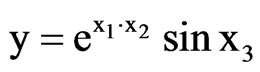
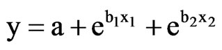 multi-exponential modeling
θ = magnitude of x-value (example)
θ1 < x < θ2 y = a1 + b1x3 spline modeling
θ2 < x < θ3 y = a2 + b2x3
θ3 < x < θ4 y = a3 + b3x3
NOTES
*Corresponding author.