American Journal of Climate Change
Vol.3 No.1(2014), Article ID:43632,17 pages DOI:10.4236/ajcc.2014.31004
Applying Downscaled Global Climate Model Data to a Hydrodynamic Surface-Water and Groundwater Model
Eric Swain1, Lydia Stefanova2, Thomas Smith3
1US Geological Survey, Florida Water Science Center, Davie, USA
2Center for Ocean-Atmospheric Prediction Studies, Tallahassee, USA
3US Geological Survey, Southeast Ecological Science Center, St. Petersburg, USA
Email: edswain@usgs.gov
Copyright © 2014 by authors and Scientific Research Publishing Inc.
This work is licensed under the Creative Commons Attribution International License (CC BY).
http://creativecommons.org/licenses/by/4.0/


Received 15 August 2013; revised 16 September 2013; accepted 14 October 2013
ABSTRACT
Precipitation data from Global Climate Models have been downscaled to smaller regions. Adapting this downscaled precipitation data to a coupled hydrodynamic surface-water/groundwater model of southern Florida allows an examination of future conditions and their effect on groundwater levels, inundation patterns, surface-water stage and flows, and salinity. The downscaled rainfall data include the 1996-2001 time series from the European Center for MediumRange Weather Forecasting ERA-40 simulation and both the 1996-1999 and 2038-2057 time series from two global climate models: the Community Climate System Model (CCSM) and the Geophysical Fluid Dynamic Laboratory (GFDL). Synthesized surface-water inflow datasets were developed for the 2038-2057 simulations. The resulting hydrologic simulations, with and without a 30-cm sea-level rise, were compared with each other and field data to analyze a range of projected conditions. Simulations predicted generally higher future stage and groundwater levels and surface-water flows, with sea-level rise inducing higher coastal salinities. A coincident rise in sea level, precipitation and surface-water flows resulted in a narrower inland saline/fresh transition zone. The inland areas were affected more by the rainfall difference than the sea-level rise, and the rainfall differences make little difference in coastal inundation, but a larger difference in coastal salinities.
Keywords:Hydrologic Models; Climate Change; Rainfall; Hydrodynamics; Salinity

1. Introduction
Numerical models are being used to simulate and predict the effects of natural and anthropogenic stressors on the hydrology and critical ecosystems. The development of advanced models that couple groundwater with surface-water while representing complex hydrodynamics and salinity transport has culminated in the Flow and Transport in a Linked Overland/Aquifer Density-Dependent System (FTLOADDS) simulator [1] . In FTLOADDS, the two-dimensional hydrodynamic surface-water flow and transport simulator SWIFT2D [2] is combined with the three-dimensional groundwater flow and salinity transport simulator SEAWAT [3] . Vertical leakage and salt flux between surface water and groundwater are computed in FTLOADDS, making a complete simulation of the hydrologic system.
The hydrodynamic surface-water formulation in SWIFT2D allows the FTLOADDS simulator to represent more rapid transients associated with tidal changes and precipitation events [4] -[9] . Transient processes, such as surface-water flooding and drying, are represented along with longer timescale processes such as evapotranspiration and groundwater responses. The evapotranspiration is computed based on the Penman-Monteith formulation coupled to the heat-transport capabilities of FTLOADDS [10] .
The FTLOADDS simulator has been applied to several south Florida regions with coastal interactions. The models developed with FTLOADDS have been used to develop insight into water management implications and planning [11] . Two models that have been constructed with FTLOADDS are the TIME model of the Everglades National Park area [12] and the BISCAYNE model of the eastern coastal area [13] (Figure 1). These two models can be simulated together, covering the tip of the Florida peninsula, and provide a useful tool to evaluate ongoing restoration efforts to better regulate the quality, quantity, timing and distribution of water flows of the south Florida eco-system and provide for water resource needs. The models also can be used to provide interpretive hydrologic information for ecologic models and water management decision making.
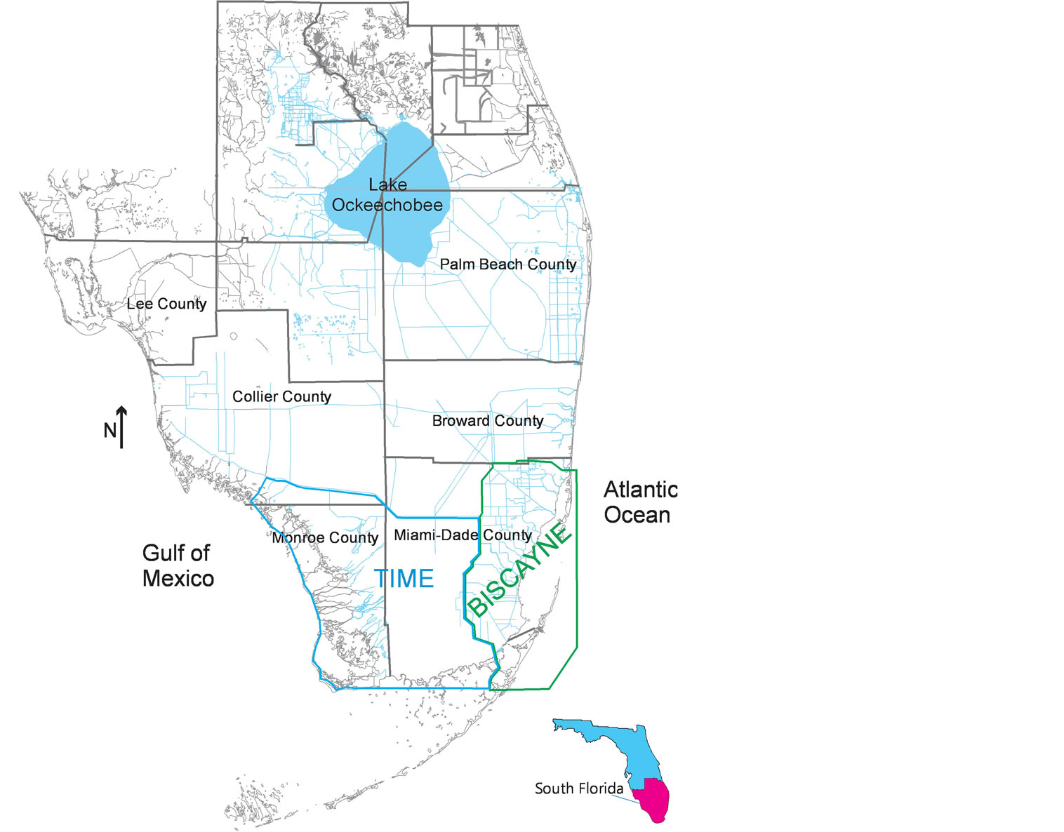
Figure 1. Locations of TIME and BISCAYNE model areas in south Florida.
A number of Global Climate Models (GCMs) have been developed to simulate global climatology including precipitation. Multiple GCMs have been used to simulate historic climate and project future climate [14] . Large-scale climate model outputs provide information for hydrologic simulations. Precipitation and temperature data from a regional climate model were used as input to four hydrologic basin models [15] . Bias correction was found to help to downscale the climate model for basin-scale modeling, but daily variability was not well reproduced. Streamflow in the Yakima River in Washington, USA, was simulated by using downscaled data from three GCMs, yielding varying degrees of agreement with field data [16] . By downscaling GCM data to the south Florida area, precipitation input data can be produced on a sufficiently small scale to describe the spatial and temporal variability relevant to the area hydrology [17] .
GCM-produced rainfall has been downscaled for areas including south Florida. The European Centre for Medium-Range Weather Forecasts (ECMWF) ERA-40 simulation is the reanalysis of historic climate information from mid-1957 to 2001 using the T159L60 version of the Integrated Forecasting System [18] . The ECMWF general circulation model consists of a dynamical component, a physical component and a coupled ocean wave component. The Community Climate System Model (CCSM) [19] was developed by the University Corporation for Atmospheric Research (UCAR). The coupled components of the CCSM include an atmospheric model (Community Atmosphere Model), a land-surface model (Community Land Model), an ocean model (Parallel Ocean Program) and a sea ice model (Community Sea Ice Model). The A2 increasing-greenhouse scenario for terrestrial carbon emissions is used [20] . The National Oceanic and Atmospheric Administration’s (NOAA) Geophysical Fluid Dynamics Laboratory (GFDL) has developed a GCM with an atmospheric physics model with tropospheric and stratospheric chemistry and has been used with varying grid resolutions [21] .
Downscaling GCM rainfall time-series input involves redistributing the precipitation volumes over a smaller grid through statistical or dynamic methods. As this process is an additional interpretation of the GCM predictions, an increase in uncertainty is anticipated. Analyses of uncertainty in statistical downscaling models indicate significant variations between stochastic and regression-based techniques [22] . Dynamic downscaling involves imbedding a smaller-scale regional climate model within the GCM [23] . This approach resolves atmospheric processes on a smaller scale and with physically consistent processes, but is computationally intensive and sensitive to the GCM boundary forcing.
Sufficient downscaled information exists from GCMs in Florida to compute evapotranspiration rates. However, analyses indicate that the downscaled solar radiation, relative humidity and wind speeds have significant biases that can produce relatively inaccurate evapotranspiration rates [24] . Consequently, the same evapotranspiration parameters used in the calibration of BISCAYNE and TIME model areas were used for the simulations in this study. The downscaled rainfall datasets were used to represent contemporary and future conditions and test the local hydrologic implications of the GCM simulations. Rainfall is a major portion of the water budget, and potential changes in rainfall rates and spatial/temporal patterns can have important implications.
This paper describes an application of downscaled GCM precipitation data [25] [26] , for historical and future conditions to develop hydrologic simulations with the BISCAYNE/TIME model. The downscaled precipitation for historical conditions (1996-2001) from the ERA-40 is used, and the resulting BISCAYNE/TIME simulation is compared with the field-data-driven BISCAYNE/TIME simulation. In addition, downscaled rainfall for historical (1996-1999) and future conditions (2038-2057) from the CCSM and GFDL models is used in BISCAYNE/ TIME. Surface-water inflow datasets are synthesized for the 2038-2057 simulations based on comparisons of existing and downscaled future rainfall volumes. The results are compared to gain insight into possible effects of climatic changes and evaluate the importance of the different GCM results.
2. Methods
The global ERA-40, CCSM, and GFDL data have been dynamically downscaled using the Scripps-Florida State University/Florida Climate Center version of the Regional Spectral Model (RSM; [25] [27] [28] . Data are downscaled for a historical period that ends in 2001 for the ERA-40 and 1999 for the CCSM and GFDL, and a future period that begins in 2038 for CCSM and GFDL. The period 2000-2037 does not have downscaled precipitation.
Bias corrections have been developed separately for the historical CCSM and GFDL rainfalls using the quantile matching approach [29] . This approach was applied to the future conditions simulations so that the differences between current and future simulated rainfalls can represent functional differences rather than inherent GCM bias.
When simulating historical hydrology, field-measured rainfall data were input to the BISCAYNE and TIME models using a 6-hour time step and spatially averaged over 8 zones [12] . Figure 2 shows the locations of rainfall stations used to develop these time series overlaid on a south Florida map with the 8 BISCAYNE and TIME mod-el rainfall zones. In contrast, the GCM simulated data were downscaled to 10 km grid points (Figure 3). In order to represent the effects of GCM-generated precipitation in the BISCAYNE/TIME models, the GCM downscaled rainfall at the 10 km points (Figure 3) was averaged within each zone to get the rainfall input dataset. This averaging was performed in the same manner for all rainfall datasets.
The time periods of the modern BISCAYNE/TIME simulations were chosen to overlap the existing field data, which are used for other (nonrainfall) hydrologic parameter time series in the simulations. The periods were:
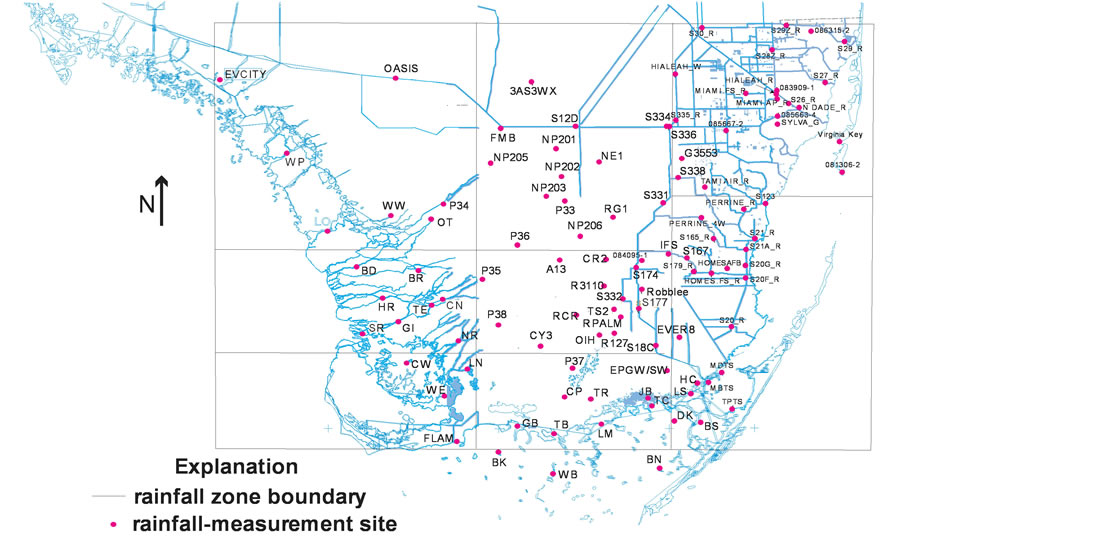
Figure 2. BISCAYNE/TIME model rainfall zones, downscaled rainfall points, and rainfall-measurement sites.
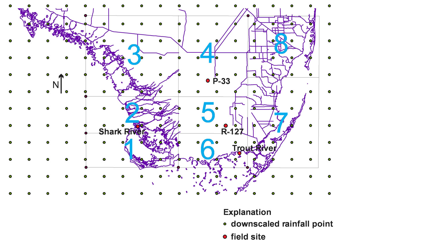
Figure 3. BISCAYNE/TIME model rainfall zones and location of field-measurement sites.
1996-2001 for the historic ERA-40 and 1996-1999 for the historic CCSM and GFDL simulations. The future conditions BISCAYNE/TIME model simulations used CCSM and GFDL downscaled rainfall and surface-water inflows synthesized for the 2038-2057 period. Tidal levels were maintained at current levels for a set of future conditions simulations and raised by 30 cm for another set of simulations. Other input data such as topography, frictional resistance, aquifer parameters, and time series of solar radiation, temperature, and canal control structure discharges were represented by the 1996-2002 data, with the time series repeated as needed to cover the 20-year period.
A future condition considered in the south Florida hydrology was change in sea level and the combined effects of changes in precipitation and sea-level rise. Scenarios with different mean sea level were simulated in BISCAYNE/TIME by adding the sea-level difference to the historical data time series uniformly. Selection of a 30-cm rise above current sea levels was considered to be a moderate estimate for the 2038-2057 period [10] . Simulating future rainfall effects with and without the sea-level rise provided a means to separately measure the relative effect of precipitation and sea level.
The hydrologic simulation using field-measured rainfall input is referred to as the BASE case. This and the other simulations are named by the rainfall data used (BASE, ERA40, CCSM, or GFDL), the simulation period (Historical or Future), and whether sea-level rise is simulated (SLR). The eight simulations are: BASEHistorical, ERA40Historical, CCSMHistorical, GFDLHistorical, CCSMFuture, GFDLFuture, CCSMFutureSLR, and GFDLFutureSLR.
2.1. Downscaled Historical Conditions
Comparing the historical-conditions cumulative rainfall by each method, averaged over the 8 rainfall zones, indicated the ERA-40 downscaled data (ERA40Historical) were significantly greater than measured values in the first year, 1996 (Figure 4). Less deviation between both was observed in subsequent years, but appeared to be most significant when specific storm events occur (for example, 10/15/1996, 6/9/1997, and markedly on 11/5/2001). This comparison indicates that major short-term storm events were not as accurately represented as long-term average precipitation. The ERA40Historical cumulative rainfall was larger than field data in all of the model zones except for zone 5 (Table 1) which is in central Everglades National Park (Figure 3).
The downscaled, cumulative CCSM historical data (CCSMHistorical) provided the best match of cumulative field volumes (Figure 4). However, this CCSMHistorical rainfall data did not demonstrate the variability of the measured data in BASEHistorical or the ERA40Historical. The CCSMHistorical total cumulative rainfall was less than the measured values in BASEHistorical in all rainfall zones with the exception of zone 3 (Table 1). This deviation largely occurred in the latter half of the 1999 (Figure 4). GFDLHistorical data did not match the total cumulative volume as well as CCSMHistorical, but did represent the variability observed in BASEHistorical
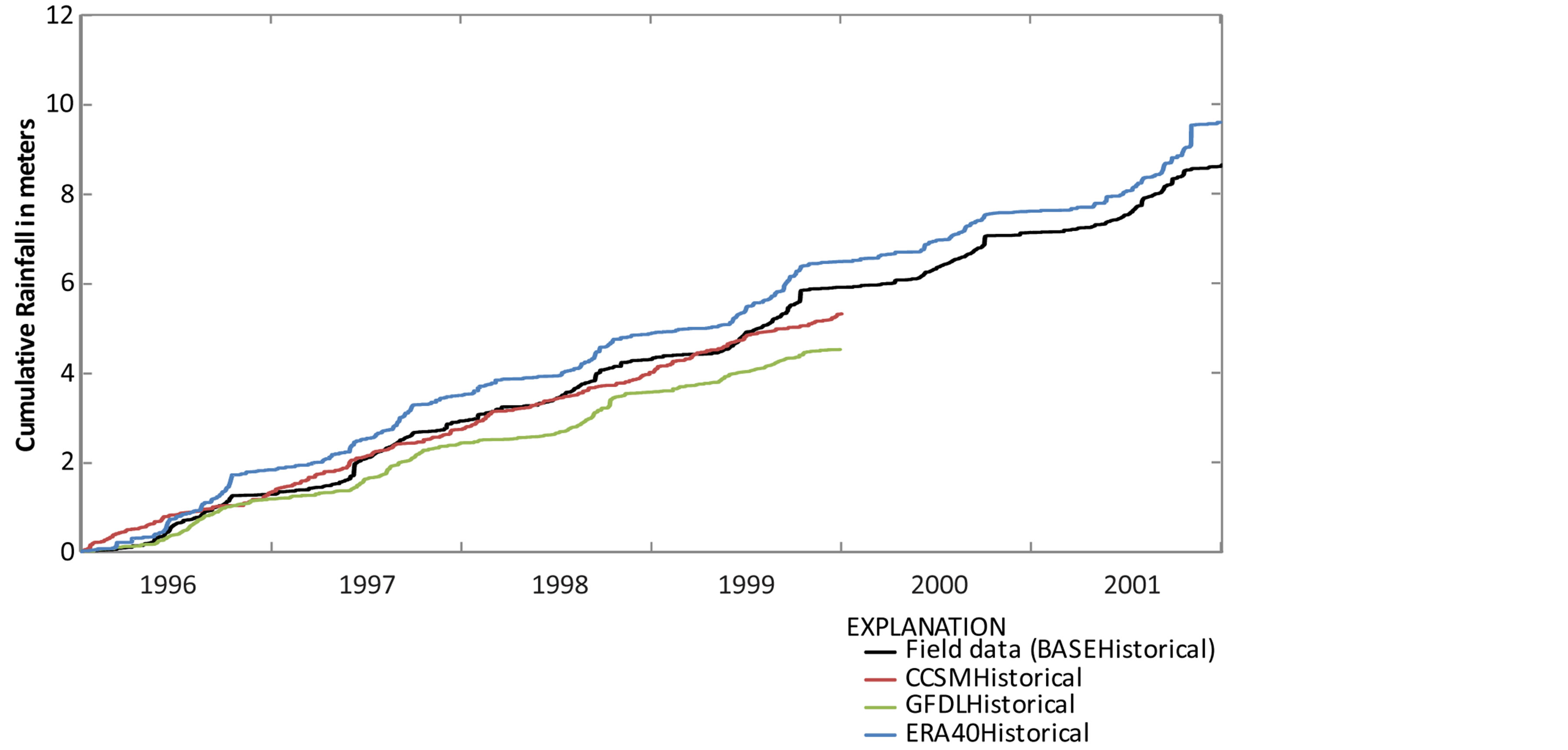
Figure 4. Cumulative rainfall from field data and downscaled climate model data.
measured rainfall better than CCSMHistorical. GFDLHistorical had the lowest total cumulative rainfall in all zones (Table 1).
2.2. Downscaled Future Conditions
A comparison of the cumulative rainfall volume between CCSMHistorical and CCSMFuture and between GFDLHistorical and GFDLFuture indicated greater future cumulative rainfall amounts (Figure 5). The tendency of CCSM to produce higher cumulative rainfall than GFDL in the historical period was also the case in the future period. Downscaled rainfall from the CCSM and CFDL GCMs were applied to delineated zones (Figure 3) to represent future hydrologic conditions in the BISCAYNE/TIME model domains.
Surface-water inflows were related to the effect of rainfall in the model area and a regulated water-delivery canal-control network. Instead of using a rainfall-runoff regression technique, which was more appropriate in higher-slope and less-controlled environments than south Florida, the surface-water inflows for CCSMFuture and GFDLFuture were synthesized by assuming a fixed relationship between cumulative inflows and rainfall. This was accomplished by converting the rainfall and surface-water inflow data from BASEHistorical and the

Table 1. Cumulative rainfall 1996-2001 in meters for BISCAYNE/TIME model zones.
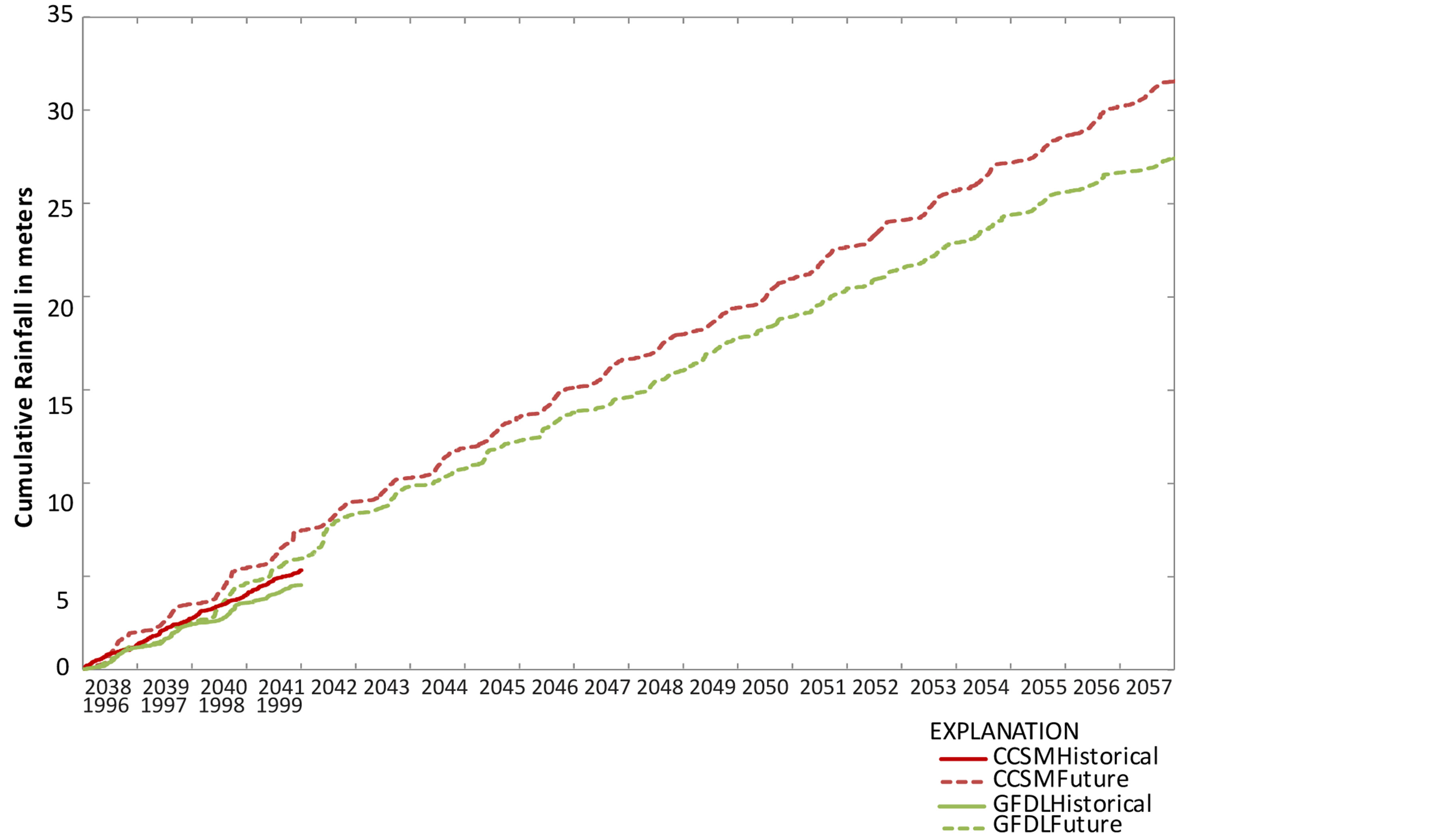
Figure 5. Cumulative historic and future rainfall from downscaled climate model data.
rainfall data from CCSMFuture and GFDLFuture to cumulative values. The BASEHistorical datasets were repeated to produce a sufficient time series to match the Future data (20 years). For each daily value of the CCSMFuture or GFDLFuture cumulative rainfall, the day of the same BASEHistorical cumulative rainfall value was located and the BASEHistorical cumulative inflow value from that day was extracted. The resulting synthesized time series of CCSMFuture and GFDLFuture cumulative inflows were then converted back to daily inflows and temporally smoothed with a 29-day moving average window.
The CCSMFuture and GFDLFuture synthesized cumulative inflow volumes (Figure 6) were seen to follow the rainfall patterns (Figure 5) as designed. As was the case with the rainfall volumes, the future inflow volumes were higher than the historical period. This method for synthesizing surface-water inflows was highly simplified, and assumed that rainfall patterns explain surface-water management operational decisions, and that this relationship would also be similar in the future. The South Florida Water Management District schedules water deliveries using a rainfall and surface-water flow regression algorithm [30] . It may be reasonable to assume such a relationship in future managed flows.
3. Results
The statistics used for comparison with field data include the root-mean square error (RMSE) and the NashSuttcliffe Efficiency (NS), each given by:
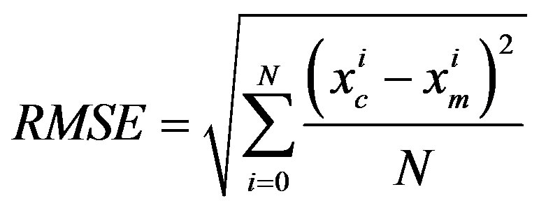 (1)
(1)
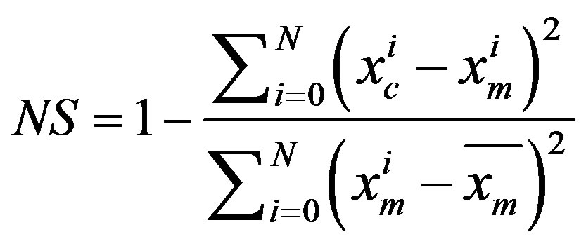 (2)
(2)
where xc is the model-computed value, xm is the field-measured value, and the overbar indicates the mean value. The RMSE measures the error in the units of the quantity analyzed, whereas the NS relates the magnitude of the error to the variability in the data. The closer the NS value is to 1, the smaller the error, with an NS value of 0 indicating that the error is as large as the variance of the measured data.
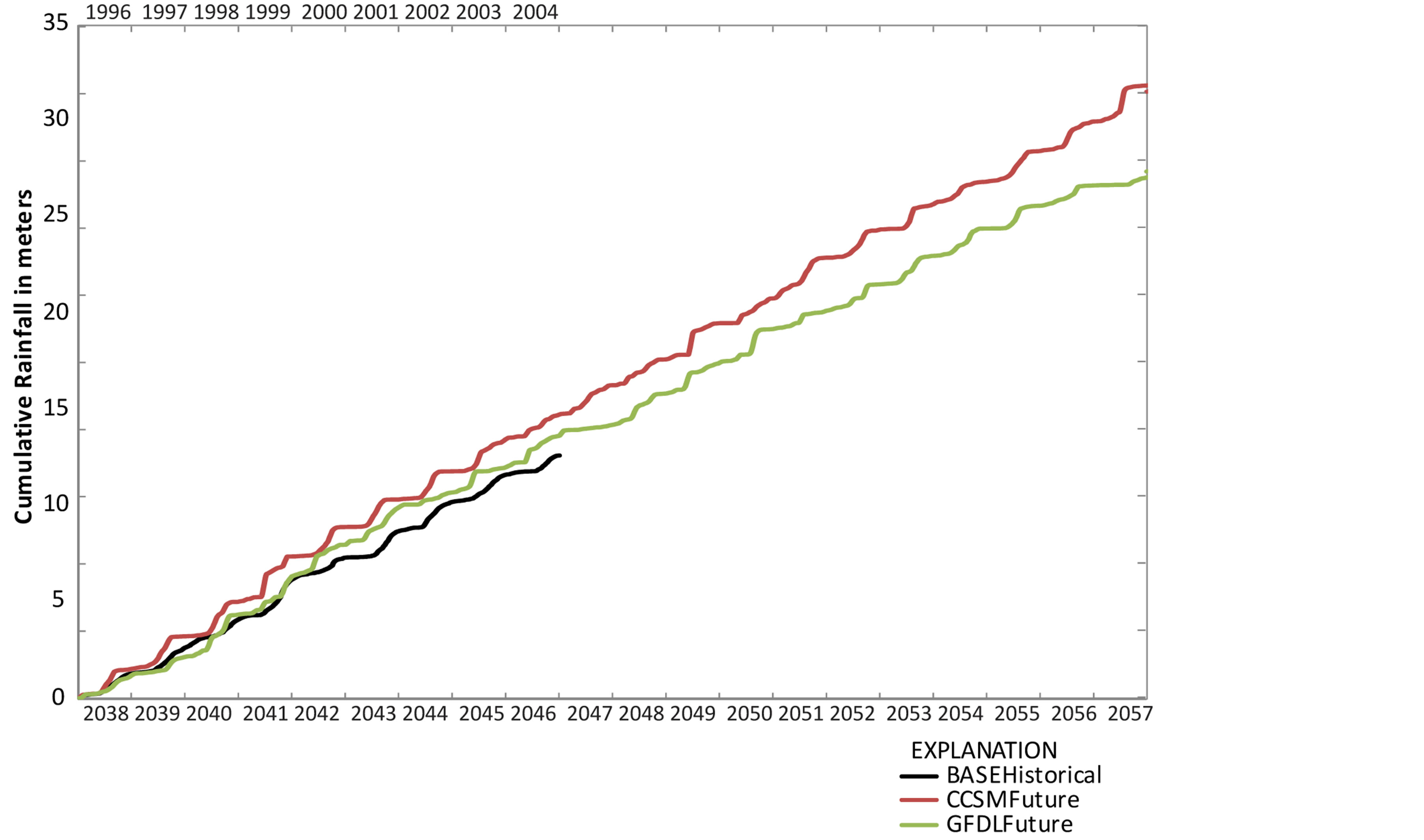
Figure 6. Cumulative historic and synthesized future surface-water inflows.
Four field sites were chosen to compare model results (Figure 3). Sites P-33 and R-127 are surface-water stage measurement sites, and Shark River and Trout River are discharge measurement sites. Surface-water simulation results were generated on a 10-minute time step with all hydrodynamic effects included; these values were averaged daily for comparison with field values.
3.1. Downscaled Historical Conditions
Rainfall data for the ERA40Historical, CCSMHistorical and GFDLHistorical simulations were input to TIME/ BISCAYNE and the simulated hydrologic output compared with the BASEHistorical simulation. None of the three simulations using downscaled rainfall from climate models (ERA40Historical, CCSMHistorical, or GFDLHistorical) produced overall results as good as the BASEHistorical (Figure 7 and Table 2). Although
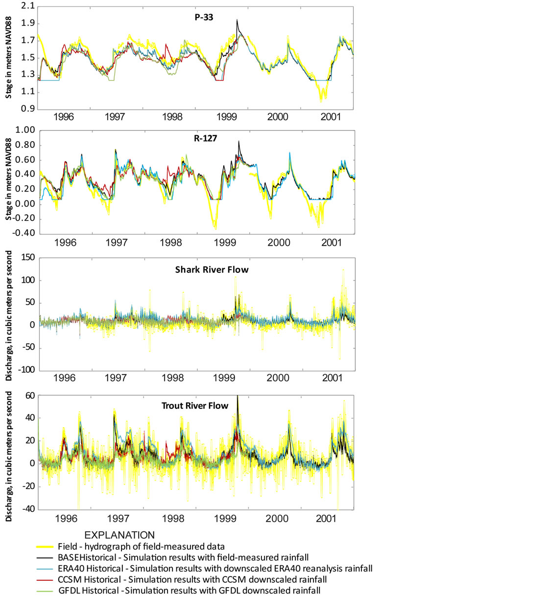
Figure 7. Measured and simulated stage and discharge at selected sites for historical simulations.
both the CCSMHistorical and GFDLHistorical simulations produced a smaller RMSE than BASEHistorical for Shark River discharge, none of the NS efficiencies for CCSMHistorical and GFDLHistorical were as satisfactory as BASEHistorical (Table 2). CCSMHistorical had a peak stage and discharge event in mid-1998 that could be observed at all four sites (Figure 7). Examination of Figure 4 indicates that the CCSMHistorical cumulative rainfall line continued to slope upward during this period, indicating continued rainfall, when all the other cumulative rainfall datasets were more horizontal.
The Trout River field site was the only location with surface-water salinity observations for the 1996-2001 period. The deviation of mid-1998 CCSMHistorical rainfall was reflected as lower salinity when compared to the other simulations (Figure 8). All simulations concurrently deviated from measured salinities, especially at the beginning of the simulation when the models’ initial conditions were dissipating.
3.2. Time Series Analyses of Historical and Future Simulations
Downscaled rainfall for the CCSMFuture and GFDLFuture simulations, with the associated synthesized surface-water inflow data, were input into the TIME/BISCAYNE simulator. The CCSMFutureSLR and GFDLFutureSLR simulations additionally included a 30-cm sea-level rise. These simulations of future conditions were compared with simulated historical conditions, both on an average daily value for an average single year (Figure 9). The CCSMFuture and CCSMFutureSLR models suggested that stage and discharge increased during south Florida’s wet season months of May through September. The CCSMHistorical and all GFDL simulations did not show this phenomenon.
It may seem counterintuitive that a 30-cm sea-level rise would increase coastal outflows at Shark and Trout Rivers, but the river overbank flow areas expand in response to a rise in sea level, increasing the effective discharge. The stages at P-33 and R-127 changed only slightly in response to sea-level rise (Figure 9), but both sites are located at a distance inland (Figure 3).
Table 2. Root Mean Square Error and Nash-Suttcliffe comparison of stage and discharge time series with field data.
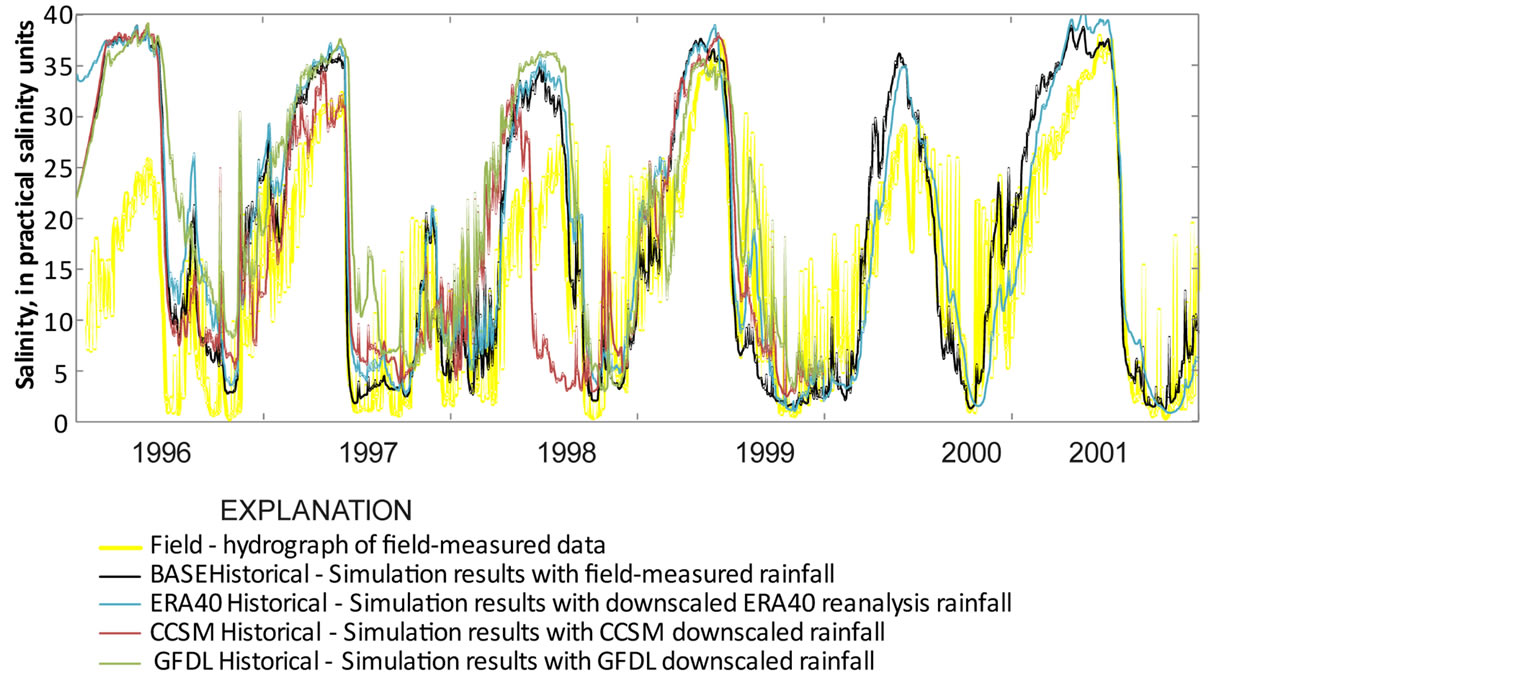
Figure 8. Measured and simulated Trout River salinities for historical simulations.
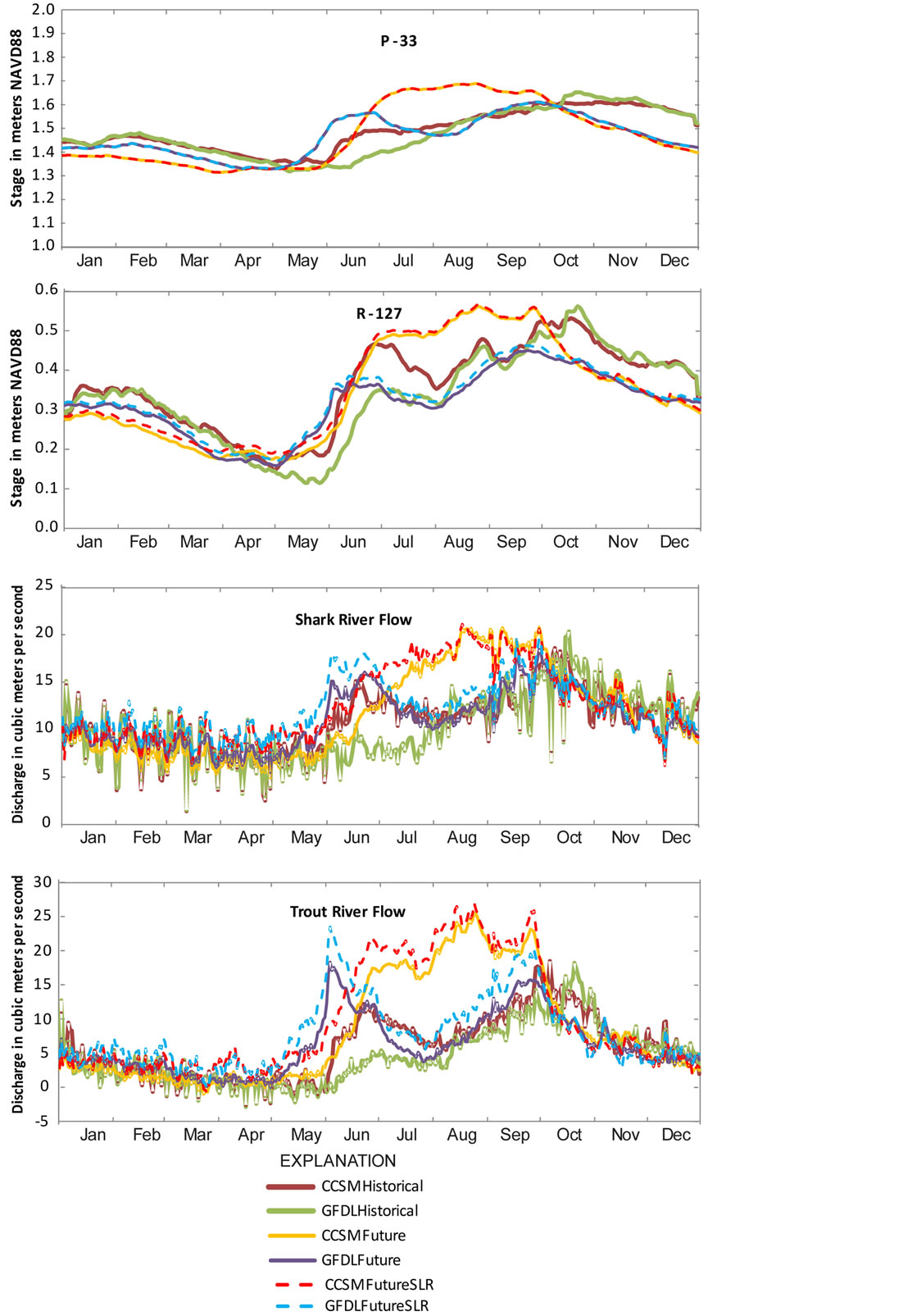
Figure 9. Average stage and discharge at selected sites for days of the year.
The variances in the stage and discharge data were consistently higher for the future-condition simulations (Table 3). However, the ERA40Historical simulation had anomalously higher variances than other historical and some future simulations. Comparisons of CCSMHistorical to CCSMFuture and GFDLHistorical to GFDLFuture indicated that stage and discharge variances increase roughly twofold in the future-conditions simulations. Less difference in variance was apparent between the future with and without sea-level rise. So the simulations suggest increased hydrologic variability in the future is due more to precipitation changes than sealevel rise.
The historical and future salinity values at Trout River were similarly compared for a single average year (Figure 10). Both the CCSM and GFDL simulations suggested Trout River will experience lower salinities in the future. The differences between the CCSM and GFDL simulations were most apparent in the July-September period, where all CCSM simulations consistently predicted lower salinities than the GFDL simulations. This time of the year corresponds to the period when the CCSM simulations produced higher stages and flows (Figure 8). Both CCSMFutureSLR and GFDLFutureSLR simulations indicated the 30-cm sea-level rise increased October-December river salinity. Rainfall diminished at this time but remnant fresh water still drained to the coast. The higher sea level facilitated the intrusion of saltwater at these times.
3.3. Spatial Analysis of Historical and Future Simulations
BISCAYNE/TIME maps showing the percent time inundated, averaged over the entire simulation period provided useful insight into wetland hydroperiods (Figure 11). Hydroperiods are important to understanding waterlevel patterns and wetland ecology. Comparisons of these maps indicated that the CCSM and GFDL simulations produced similar trends in inundation. The sea-level rise effects were most dramatic along the western and southern Everglades National Park coastlines. The effects of precipitation pre-dominated over sea-level change in inland areas.
The difference in inundation between historic and future scenarios had significant spatial variability (Figure 12).
Table 3. Variances of stage and discharge time series.
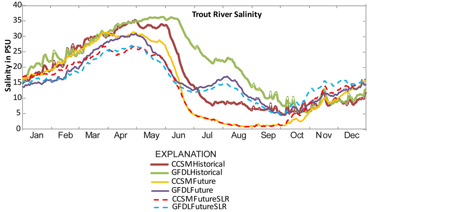
Figure 10. Average trout river salinities for days of the year.
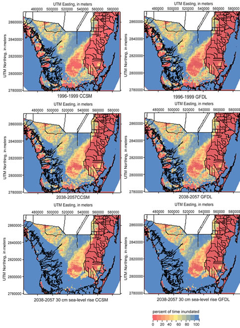
Figure 11. Percent of time inundated using CCSM and GFDL downscaled rainfall for 1996-1999 (Historical) and 2038-2057 (Future) simulations with and without 30 cm sea-level rise (SLR).
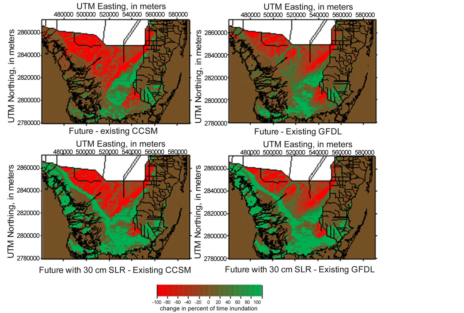
Figure 12. Difference in percent of time inundated using CCSM and GFDL downscaled rainfall 1996-1999 (Historical) and 2038-2057 (Future) simulations with and without 30 cm sea-level rise (SLR).
Elevated topographic areas in the center of the model area were inundated more frequently in the future whereas lower topographic areas to the north and central south were inundated less often. This scenario was a consequence of the higher temporal variability in stages (Table 3), which caused rarely inundated areas to inundate more often and frequently inundated areas to dry more often. Less difference in inundation was seen nearer to the coast when the future scenarios did not include simulation of sea-level rise (Figure 12), but a combination of future precipitation and higher sea level produced a higher contrast in inundation periods between the coastal and inland areas.
Simulated surface-water salinity for each scenario was averaged over the entire simulation to examine hydrologic system response to changes in rainfall and sea level (Figure 13). Both the CCSM and GFDL simulations showed similar trends. Assuming no rise in sea level, with the predicted increase in precipitation, the future surface-water salinities were substantially lower in southernmost coastal areas, but less so along the western coast. Simulation of a 30-cm sea-level rise increased the future western coastal salinity but the southern coastal salinity was still less than the historical simulation. These results indicated that the combination of future rainfall and sea-level rise created a narrower transition zone from seawater salinity to fresh water (Figure 13).
4. Summary and Conclusions
Global Climate Model (GCM) output was utilized to create downscaled rainfall data input to the BISCAYNE/ TIME model. The simulations compared included the Medium-Range Weather Forecasts (ECMWF) ERA-40 downscaled data for the period 1996-2001, the Community Climate System Model (CCSM) simulations for 1996-1999 and 2038-2057, and the Geophysical Fluid Dynamic Laboratory (GFDL) simulations for 1996-1999 and 2038-2057. The historical conditions of measured rain-fall base BISCAYNE/TIME simulation, and fieldmeasured stage, discharge, and salinity data were used for comparison. These simulations were respectively referred to: ERA40Historical, CCSMHistorical, CCSMFuture, GFDLHistorical, GFDLFuture and BASEHistorical. Comparison of ERA40Historical, CCSMHistorical, and GFDLHistorical with field-measured data indicated
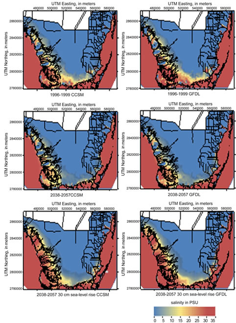
Figure 13. Salinity distributions averaged over the entire simulation periods for differing CCSM and GFDL downscaled rainfalls and sea levels.
that the downscaled rainfall produced similar results but not as well as BASEHistorical. CCSMHistorical deviated from the base simulation more than GFDLHistorical, especially in the mid-1998 time period.
Future-condition rainfall for the years 2038-2057 was downscaled from the CCSM and GFDL GCM models and resolved for the BISCAYNE/TIME rainfall input zones. The rainfall produced by both GCM models for future 2038-2057 conditions had a significantly higher average rate than their corresponding historical simulations. Surface-water flow boundary datasets for the CCSMFuture and GFDLFuture simulations were developed from historical-conditions flow and the relation between the historical conditions and the CCSMFuture and GFDL Future conditions rainfall.
Water-level and discharge, salinity time series, inundation times and average salinity values were compared between simulations. The water levels and discharge in CCSMFuture were significantly higher than that in CCSMHistorical in the July-September period, but the GFDLHistorical and GFDLFuture simulations did not indicate such a dramatic difference. Both sets of simulations indicated that the future rainfall changes induced higher variability in hydrologic conditions, causing higher topographic areas to inundate more often and lower topographic areas to dry out more often. The two future scenarios were combined with a simulated 30-cm sea-level rise. The combined effects produced higher inundation for most of the model areas except for the farthest inland areas. This scenario resulted in a narrower simulated transition area between the saline zone and inland fresh water.
The differences in rainfall under current and GCM predicted future conditions induce changes in the surface-water salinity and water-level regimes. General conclusions are difficult to formulate because of the various lengths of the simulations: 7 years for BASEHistorical, 4 years for the GCM-driven Historical runs, and 20 years for the GCM-driven Future runs. Longer-term simulations would be necessary to establish an average effect on the climatic changes. Simulation results also indicated that both rainfall changes and sea-level rise were important factors affecting flows and inundation. Inland areas were predominantly affected by rainfall variations and coastal areas by sea-level changes. The salinity transition zone was squeezed between these two effects.
Acknowledgements
This research was supported by the U.S. Geological Survey (USGS) projects: La Florida—A Land of Flowers on a Latitude of Deserts; and, FISCHS-Past and Future Impacts of Sea Level Rise on Coastal Habitats and Species. Funding from the USGS National Climate Change and Wildlife Science Center and the USGS Ecosystems Program are gratefully acknowledged. The authors thank personnel at the Center for Ocean-Atmospheric Prediction Studies at Florida State University including Assistant Professor Vasu Misra for climate model data development and Climate Data Analyst Steven DiNapoli for the bias-correction calculations. Additionally, discussions with collaborators from the Florida Coastal Everglades Long-Term Ecological Research (FCE-LTER) program are acknowledged. The FCE-LTER is funded under National Science Foundation Grant No. DEB- 9910514. Comments from two anonymous reviewers improved the manuscript.
References
- Langevin, C.D., Swain, E.D. and Wolfert, M.A. (2005) Simulation of Integrated Surface-Water/ Ground-Water Flow and Salinity for a Coastal Wetland and Adjacent Estuary. Journal of Hydrology, 314, 212-234. http://dx.doi.org/10.1016/j.jhydrol.2005.04.015
- Swain, E.D. (2005) A Model for Simulation of Surface-Water Integrated Flow and Transport in Two Dimensions: SWIFT2D User’s Guide for Application to Coastal Wetlands. U.S. Geological Survey Open-File Report 2005-1033, 88 p.
- Langevin, C.D., Thorne Jr., D.T., Dausman, A.M., Sukop, M.C. and Guo, W.X. (2007) SEAWAT Version 4: A Computer Program for Simulation of Multi-Species Solute and Heat Transport. U.S. Geological Survey Techniques and Methods Book 6, Chapter A22, 39 p.
- Bales, J.D. and Robbins, J.C. (1995) Simulation of Hydrodynamics and Solute Transport in the Pamlico River Estuary, NC. US Geological Survey Open-File Report 94-454, 85 p.
- Goodwin, C.R. (1987) Tidal-Flow, Circulation, and Flushing Changes Caused by Dredge and Fill in Tampa Bay, Florida. US Geological Survey Water-Supply Paper 2282, 88 p.
- Goodwin, C.R. (1991) Tidal-Flow, Circulation, and Flushing Changes Caused by Dredge and Fill in Hillsborough Bay, Florida. US Geological Survey Water-Supply Paper 2376, 49 p.
- Goodwin, C.R. (1996) Simulation of Tidal-Flow, Circulation, and Flushing of the Charlotte Harbor Estuarine System, FL. US Geological Survey Water-Resources Investigations Report 93-4153, 92 p.
- Leendertse, J.J., Langerak, A. and de Ras, M.A.M. (1981) Two-Dimensional Tidal Models for the Delta Works. In: H. B. Fischer, Ed., Transport Models for Inland and Coastal Waters, Proceedings of a Symposium on Predictive Ability. Academic Press, New York, 408-450.
- Robbins, J.C. and Bales, J.D. (1995) Simulation of Hydrodynamics and Solute Transport in the Neuse River Estuary, NC. US Geological Survey Open-File Report 94-511, 85 p.
- Swain, E.D. and Decker, J.D. (2010) A Measurement-Derived Heat-Budget Approach For Simulating Coastal Wetland Temperature with a Hydrodynamic Model. Wetlands, 30, 635-648. http://dx.doi.org/10.1007/s13157-010-0053-7
- Swain, E.D., Lohmann, M. and Decker, J.D. (2008) Hydrologic Simulations of Water-Management Scenarios in Support of the Comprehensive Everglades Restoration Plan. The Role of Hydrology in Water Resources Management: IAHS Red Book Series, UNESCO/IAHS Symposium, Napoli.
- Wang, J.D., Swain, E.D., Wolfert, M.A., Langevin, C.D., James, D.E. and Telis, P.A. (2007) Applications of Flow and Transport in a Linked Overland/Aquifer Density Dependent System (FTLOADDS) to Simulate Flow, Salinity, and Surface-Water Stage in the Southern Everglades, Florida. U.S. Geological Survey Scientific Investigations Report 2007-5010, 90 p.
- Lohmann, M.A., Swain, E.D., Wang, J.D. and Dixon, J. (2012) Evaluation of Effects of Changes in Canal Management and Precipitation Patterns on Salinity in Biscayne Bay, Florida, Using an Integrated Surface-Water/Groundwater Model. U.S. Geological Survey Scientific Investigations Report 2012-5099, 94 p.
- Intergovernmental Panel on Climate Change (2007) Climate Change 2007-The physical science basis. In: S. Solomon, D. Qin, M. Manning, Z. Chen, M. Marquis, K. B. Averyt, M. Tignor and H. L. Miller, Eds., Contribution of Working Group I to the Fourth Assessment Report of the Intergovernmental Panel on Climate Change, United Kingdom, Cambridge University Press, Cambridge.
- Hay, L.E., Clark, M.P., Wilby, R.L., Gutowski, W.J., Leavesley, G.H., Pan, Z., Arritt, R.W. and Takle, E.S. (2002) Use of Regional Climate Model Output for Hydrologic Simulations. Journal of Hydrometeorology, 3, 571-590. http://dx.doi.org/10.1175/1525-7541(2002)003<0571:UORCMO>2.0.CO;2
- Salathe, E.P. (2005) Downscaling Simulations of Future Global Climate with Application to Hydrologic Modelling. International Journal of Climatology, 25, 419-436. http://dx.doi.org/10.1002/joc.1125
- Obeysekera, J., Irizarry, M., Park, J., Barnes, J. and Dessalegne, T. (2011) Climate Change and Its Implication for Water Resources Management in South Florida. Journal of Stochastic Environmental Research & Risk Assessment, 25, 495. http://dx.doi.org/10.1007/s00477-010-0418-8
- Uppala, S.M., KÅllberg, P.W., Simmons, A.J., et al. (2005) The ERA-40 Re-Analysis. Quarterly Journal of the Royal Meteorological Society, 131, 2961-3012. http://dx.doi.org/10.1256/qj.04.176
- Collins, W.D., Bitz, C.M., Blackmon, M.L., et al. (2006) The Community Climate System Model Version 3 (CCSM3). Journal of Climate, 19, 2122-2143. http://dx.doi.org/10.1175/JCLI3761.1
- Hoffman, F.M., Fung, I., Randerson, J., Thornton, P., Stockli, R., Heinsch, F., Running, S., Hibbard, K., John, J., Covey, C., Foley, J., Post, W.M., Hargrove, W.W., Erickson, D.J. and Mahowald, N. (2006) Preliminary Results from the CCSM Carbon-Land Model Intercomparison Project (C-LAMP). Eos Trans. AGU, 87(52), Fall Meet. Suppl., Abstract B51C-0316.
- Zhao, M., Held, I.M., Lin, S.-J. and Vecchi, G.A. (2009) Simulations of Global Hurricane Climatology, Interannual Variability, and Response to Global Warming Using a 50-km Resolution GCM. Journal of Climate, 22, 6653-6678. http://dx.doi.org/10.1175/2009JCLI3049.1
- Etemadi, H., Samadi, S. and Sharifikia, M. (2013) Uncertainty Analysis of Statistical Downscaling Models Using General Circulation Model over an International Wetland. Climate Dynamics. http://dx.doi.org/10.1007/s00382-013-1855-0
- Fowler, H.J., Blenkinsop, S. and Tebaldi, C. (2007) Linking Climate Change Modeling to Impacts Studies: Recent Advances in Downscaling Techniques for Hydrological Modeling. International Journal of Climatology, 27, 1547-1578. http://dx.doi.org/10.1002/joc.1556
- Obeysekera, J. (2013) Validating Climate Models for Computing Evapotranspiration in Hydrologic Studies: How Relevant Are Climate Model Simulations over Florida? Regional Environmental Change, 13, 81-90. http://dx.doi.org/10.1007/s10113-013-0411-0
- Stefanova, L., Misra, V., Chan, S.C., Griffin, M., O’Brien, J. and Smith III, T.J. (2012) A Proxy for High-Resolution Regional Reanalysis for the Southeast United States: Assessment of Precipitation Variability in Dynamically Downscaled Reanalyses. Climate Dynamics, 38, 2449-2466. http://dx.doi.org/10.1007/s00382-011-1230-y
- Stefanova, L., Misra, V. and Smith III, T.J. (2012) Climate Means, Trends and Extremes in the Everglades: Historical Data and Future Projections. 9th INTECOL International Wetlands Conference, Orlando, 3-8 June 2012.
- Kanamaru, H. and Kanamitsu, M. (2007) Scale-Selective Bias Correction in a Downscaling of Global Analysis Using a Regional Model. Monthly Weather Review, 135, 334-350. http://dx.doi.org/10.1175/MWR3294.1
- Misra, V., Moeller, L., Stefanova, L., Chan, S., O’Brien, J.J., Smith III, T.J. and Plant, N. (2011) The Influence of Atlantic Warm Pool on Florida Sea Breeze. Journal of Geophysical Research: Atmospheres, 116, Article ID: D00Q06.
- Wood, A.W., Maurer, E.P., Kumar, A. and Lettenmaier, D. (2002) Long-Range Experimental Hydrologic Forecasting for the Eastern United States. Journal of Geophysical Research, 107, 4429. http://dx.doi.org/10.1029/2001JD000659
- Weaver, J., Brown, B., Browder, J., Kitchens, W., Wesley, D., Burns, L., Scheidt, D., Ferrell, D., Thompson, N., Ogden, J., Armentano, T., Robblee, M., Loftus, W., Glaz, B. and Ortner, P. (1993) Federal Objectives for the South Florida Restoration by the Science Sub-Group of the South Florida Management and Coordination Working Group. South Florida Restoration Science Subgroup. http://www.sfrestore.org/sct/docs/subgrouprpt/index.htm