American Journal of Climate Change
Vol.1 No.3(2012), Article ID:22477,4 pages DOI:10.4236/ajcc.2012.13013
Restoration of Time-Spatial Scales in Global Temperature Data
Department of Epidemiology and Biostatistics, State University of New York at Albany, New York, USA
Email: *mluo@albany.edu
Received June 21, 2012; revised July 25, 2012; accepted August 11, 2012
Keywords: Separation of Scales; Kolmogorov-Zurbenko Filtration in Time and Space; Climate Variability; El Niño-Like Movement; Global Long Term Trend; Spectral Analysis; Correlation Analysis; Temporal-Spatial Data
ABSTRACT
The objective of this paper is to utilize images of spatial and temporal fluctuations of temperature over the Earth to study the global climate variation. We illustrated that monthly temperature observations from weather stations could be decomposed as components with different time scales based on their spectral distribution. Kolmogorov-Zurbenko (KZ) filters were applied to smooth and interpolate gridded temperature data to construct global maps for long-term (≥ 6 years) trends and El Niño-like (2 to 5 years) movements over the time period of 1893 to 2008. Annual temperature seasonality, latitude and altitude effects have been carefully accounted for to capture meaningful spatiotemporal patterns of climate variability. The result revealed striking facts about global temperature anomalies for specific regions. Correlation analysis and the movie of thermal maps for El Niño-like component clearly supported the existence of such climate fluctuations in time and space.
1. Introduction
The general feature of the global climate variability is an important topic for climate researchers. The past decades had seen tremendous progress in developing consistent database of meteorological observations covered long time periods [1-4]. These works generally involved assimilating, gridding and interpolating surface climate records to form a unified temperature field covering the land area of the Earth. The availability of these datasets facilitates revealing and visualizing the climate movement at the global level. By utilizing one of the datasets, we built a fine-resolution description of the mean states and space-time fluctuations of the global climate to illustrate the basic pattern of climate movement. Compared to other existing “reanalysis” works [5], our approach is more spatial-temporal statistics oriented in that we decomposed climate movements into independent temporal and spatial components on different scales based on the feature of the data. The spatial-temporal approach provides a solid base and can serve for a number of applications in the future.
Our work focused on surface temperature, the most important role in investigating the global or regional climate change [6]. From the energy balance perspective, the temperature change follows the change of energy input for a specific area. For example, it was found that long-term sea-level mean temperatures were well associated with solar insolation records for the continental areas where the advection effects can be averaged out or negligible [7]. This means that we can model the energy distribution over time and space with surface temperature [8]. To this end, all observed temperature have to be adjusted to sea-level potential temperature.
From the statistical perspective, to build the profile of global climate is a typical space-time modeling task. The major challenge is the complex spatiotemporal dependencies over multiple time and spatial scales [9,10]. The presence of various scales of motion in time and space complicates the analysis and interpretation of the data [11,12]. Therefore, the first step to solve the problem should be decomposing meteorological data into components that we are interested in [13]. Based on previous study [11] and spectral analysis of the data, we choose to exam long-term (≥6 years) temperature trend and shortterm (2 to 5 years) temperature variation (El Niño-like) for gridded cells on a geographic scale of 1˚ × 1˚ (latitude times longitude). Such approach is going in line with OECD recommendation about cyclical component in time series [14].
The long-term trend and El Niño-like component usually have relative smaller amplitudes compared with seasonal temperature changes and cannot be observed directly. To separate out those data components, we introduced the Kolmogorov-Zurbenko filter (KZ) [15]. KZ filter is a local nonparametric smoothing algorithm. It has powerful capability to precisely reconstruct signals buried in high background noises. KZ filters’ outputs enabled us to visualize spatial temperature changes over time with movies of thermal maps.
The following sections describe the construction of the long-term component and El Niño-like movement of surface climate over global land areas for the period of 1893 to 2008. We will demonstrate how the long-term component movie facilitates capturing the spatial pattern of energy input and distribution over the globe land, and how the movie for El Niño-like movement helps to understand the short term temperature fluctuation and its spatial feature. The correlation analysis over these climate components revealed striking spatial/temporal correlation patterns and will also be discussed.
2. Method
2.1. Data Source and Preparing
The data source for our study is the station-based monthly mean temperature data (version 3) from the Global Historical Climate Network Dataset (GHCN) (http://www. ncdc.noaa.gov/ghcnm/v3.php). GHCN updates this dataset daily to accommodate the newest observations; and all the data have been adjusted for homogeneity and quality control [4]. Considering the data coverage, we utilized the monthly means for the period of 1890 to 2011 in our study.
GHCN collects monthly mean temperature records from about 7280 stations around the world. However, these weather stations are not evenly distributed. More specifically, there are more stations in developed countries or areas with high population density. It may enlarge the bias caused by civilization [16] if we use the station data directly. Therefore, we aggregated the station records on the latitude-longitude grid with 1˚ × 1˚ resolution by averaging the temperature records of all stations in each grid cell. The altitude of each grid cell is the mean altitude for stations within the cell. The gridded dataset avoids inadequate spatial sampling and covers most land surface except Antarctic.
The gridded monthly temperature data can be decomposed temporally and spatially. The following sections will address the separation of major spatial variations in the first place. After that, we will describe the method to identify and generate temporal components based on spectral analysis.
2.2. Latitude Pattern of Long Term Mean Temperature
Raw temperature data has strong variations along latitude and altitude. To reasonably visualize long-term global fluctuation in space, we need to remove these effects. Following paper [17], we utilized the cosine-square law to approximate the latitude pattern of long-term mean temperature:
 (1)
(1)
where  is the sea-level long-term mean temperature on latitude y. The cosine-squared term in this formula can be explained by the product of two cosine factors. The first one is the energy density for a given sunlight beam spread on unit ground square—suppose the sun is strait up on the equator (the annual average position of the sun)—this value is proportional to the cosine of latitude. The second cosine factor is the reverse of distance in the atmosphere passed through by the sunlight before it reaches the ground. The distance is proportional to the reverse of cosine of latitude, and the double reverse determines the energy volume for a sunlight beam carried to the ground and acts as the second factor of cosine.
2.3. Long Term Lapse Rate of Temperature
Temperature pattern along altitude is another spatial variation need to be addressed. Theoretically, we can convert station temperature to sea-level potential temperatures if we know station altitude and lapse rate (i.e., the rate at which temperature declines with altitude near the ground surface). However, lapse rate varies seasonally, diurnally, and regionally due to its dependence on humidity, pressure, topography, albedo, etc. The notion of constant lapse rate is an approximate description for average situation over a relative large time-space scale.
As a common practice in this area, the constant lapse rates can be calculated by regressing station temperature data on station latitudes and altitudes [7,18,19]. However, this method tends to underestimate the lapse rate value [20]. We found that the bias was caused by the extremely uneven distribution of the station observations on different altitude levels. Thus we decided to perform the regression on latitudes-altitudes grid (1˚ × 50 m), instead of stations, to avoid this problem. Along this line, the latitudes-longitude gridded data in Section 2.1 was further aggregated to latitudes-altitudes grid by averaging temperature data for all available years and stations for given latitude and altitude level, and then be regressed on the grid latitudes and altitudes to estimate the lapse rate. The rationale for this improvement rooted from our understanding of the constant lapse rate, and its result is superior to the original method.
2.4. Spatial Interactions in the Regression Model
Beside the cosine-square pattern and altitude effect of global temperature distribution, there are several other factors also need to be controlled for. First, temperature in Antarctic is lower than the value predicted by the cosine-square law, and the plateau area in Antarctic has much higher lapse rate compared with other areas. The lapse rate for tropical region near equator also needs special treatment, although it is not as high as in Antarctic [8, 21]. Additionally, temperature in the south hemisphere tends to be slightly lower than the same latitude area in the north hemisphere. To address all of these spatial variations and interactions, the linear regression model in Equation (1) was extended as Equation (2).
 (2)
(2)
where  is the sea-level mean temperature on latitude y and altitude l. S and E is the dummy variable for Antarctic (y < 70˚) and equator (−10˚ < y < 10˚), respectively. Symbol “:” represents interaction between variables. Here,
  is used to adjust the average temperature in south hemisphere; –a2 is the average lapse rate, –a5, –a6 and –a7 are the lapse rate adjustments in south hemisphere, Antarctic and equator regions. The spatial component represented by estimated coefficients (a0 to a7) and related variables will be used to adjust the station observations when we apply KZ filters to generate long term singles. The total R2 for Equation (2) is about 0.95. The cosine-square term contributed most of the R2 (0.82); altitude added another 0.1 on this base; all other terms and interactions provided some extra improvement. This fact clearly shows that the cosine-square law is the most dominating factor for temperature distribution on the Earth surface. Still cosine-square law alone makes strong exaggerations in the images of elevated areas, so clear understanding of fluctuations of global temperature in space requests to include altitude factor.
This step allows us to get rid of non-interested spatial variations and uncover the long term temperature fluctuation patterns in space and time. In the result section, we will illustrate thse patterns as thermal maps of long term temperature anomaly for different area and time period.
2.5. Spectral Analysis
On the time dimension, the manifest feature of monthly temperature data is the seasonal fluctuation with a cycle of 12 months. Usually the annual movements are more than 50 times stronger than signals in other frequency. Similar to the spatial variations, we need to remove this dominant variation to uncover other temporal components. The spectral feature of those temporal components therefore needs to be identified first. This can be done systematically based on spectral analysis with bootstrapping on KZ periodogram (KZP) [15].
KZ periodogram has strong power to separate frequencies of signals and smooth out noises. It also has the advantage to eliminate the impact of nonstationarity [15]. We utilized it in the bootstrapping of spectrum for temperature data over the globe. The steps for the spectral analysis are as following:
1) Randomly select 3000 stations over the globe;
2) For all stations with 50+ year records, calculate 5% DZ smoothed KZ periodogram over (0, 0.06);
3) Evenly divide (0, 0.06) as 133 bins, calculate the mean values of smoothed KZ periodogram on the 133 bins as the global raw periodogram;
4) Smooth the global raw periodogram with 7% DZ smoothing level.
The final periodogram (Figure 1) is the average spectral distribution for most stations on the Earth. It is consistent with the spectral analysis of the 350-year long historical Central England temperature (CET) time series [17]. The periodogram suggests that temperature variations on different places have common spectral components.
2.6. Temporal Decomposition of the Data
We utilized Kolmogorov-Zurbenko filter (KZ) [15,22-24] as the interpolation model [25] and the tool to separate components with different scales. For w-dimensional input X and smoothing window m = (m1, m2, ···, mw), k iterations of the KZ operation is represented as:

Figure 1. Average spectrum distribution for stations over the globe. The area with shadow is the cut-off separation range for long-term and El Niño-like component.
 (3)
(3)
On the time dimension, m and k should be selected according to the spectra distribution of the data. Based on the average periodogram of station data (Figure 1), we identified several components with different frequency ranges: Long-term scales (frequency < 0.012 c/m (cycles/ month)), corresponding to a period of longer than 6 or 7 years; and, shorter scales (frequency 0.017 - 0.056 c/m), corresponding to a period of 1.5 to 5 years. They can be attributed to the long-term global activity and the El Niño-like phenomenon, referred as G and E, respectively. Since the short-term fluctuation (frequency ≥ 0.0833 c/m) is not the focus in this study, our design should be able to suppress the annual movement to less than 1/2 fraction of one percent. Let’s consider the KZ filter in the following equation:
 (4)
(4)
If we set the cut-off level as half of the amplitude of output signal, the cut-off frequency for KZ25,5 is 0.0114 c/m [15], corresponding to 7.3 years cycle length. This will provide exact separation for global long-term component at each grid cell.
To generate the El Niño-like component, consider the combination of KZ filters as following:
 (5)
(5)
The cut-off frequencies for this equation are 0.01736 (c/m) on the left side, and 0.05556 (c/m) on the right side, corresponding to 4.8 years and 1.5 years, respectively. The leaking on annual frequency is only 0.26% and is negligible. Equation (5) will work well for El Niño-like signal on each grid cell.
Please note that we didn’t use  in Equation (5). This means that the cut-off frequencies for (4) and (5) are different, and the frequencies within this range (4.8 to 7.3 years cycle length) wouldn’t be included in neither E nor G. The purpose of this design is to prevent the mixing of long-term and El Niño-like movement. Since this frequency range is not the common spectral component of global temperature records (Figure 1), we can use it as a “buffer zone” between the major components that we are interested in.
2.7. Spatial Smoothing of the Components
Next we will generate the final global long-term component G and El Niño-like component E by spatially interpolating the results of the previous section with KZ filters. In Section 2.2 to 2.4, we had already got rid of the major spatial variation by removing the long-term temperature latitude pattern and altitude effect. Now we can treat the data as isotropic and spatially smooth it with same parameters. This means that the spatial filter evenly smoothed temperature records of all the grids in space, including grids with missing data. Therefore, for the result components, the investigated temperature is proportional to physical energies in time and space.
Suppose G and E are spatially smoothed signals of G and E, we have:
 (6)
(6)
 (7)
(7)
where E is as in Equation (5), but usually will be enlarged to counterbalance its amplitude attenuation. Since KZ is linear filter, it is no problem for operations in (6) and (7). Here, the spatial smoothing parameter is 3˚ × 3˚ iterated 5 times, corresponding to a critical region of  [15,26]. Considering the average correlation coefficient of temperature anomaly remains above 0.5 to distances of 1200 km for most latitudes [5], this parameter sounds like a reasonable choose.
For both long-term component G and El Niño component E, we had made movies for their thermal plots evaluated over time. This was implemented with slides generated by R lattice package on global map, aimed to visualize their correlation pattern over time and space, and facilitate capturing important events of global climate change.
2.8. Correlation Analysis
We applied correlation analysis on the generated long term component G and El Niño-like component E with a re-sampling scheme:
1) For each pair of randomly selected grid points, the correlation coefficient for their time series data over common time period was calculated;
2) Draw scatter-plot for the distance-correlation relationship based on more than 10,000 samples; same for angle-correlation relationship;
3) Applied KZ filter on distance-correlation data with parameter m = 300 and k = 3; plotted the relationship;
Since we had removed the major variation on spatial dimensions for G and E, the correlation patterns are expected to be the same on all directions. Correlation analysis results verified this assumption as well as the spatial smoothing parameters used in the previous section.
3. Results
3.1. Basic Features of the Components
We checked the spectral structure of component G and E as a verification of our design. KZ filters separated the two components as desired, and there is no signal leaking around annual frequency. Figure 2 exhibits the time series plots of those components. Please note that the long
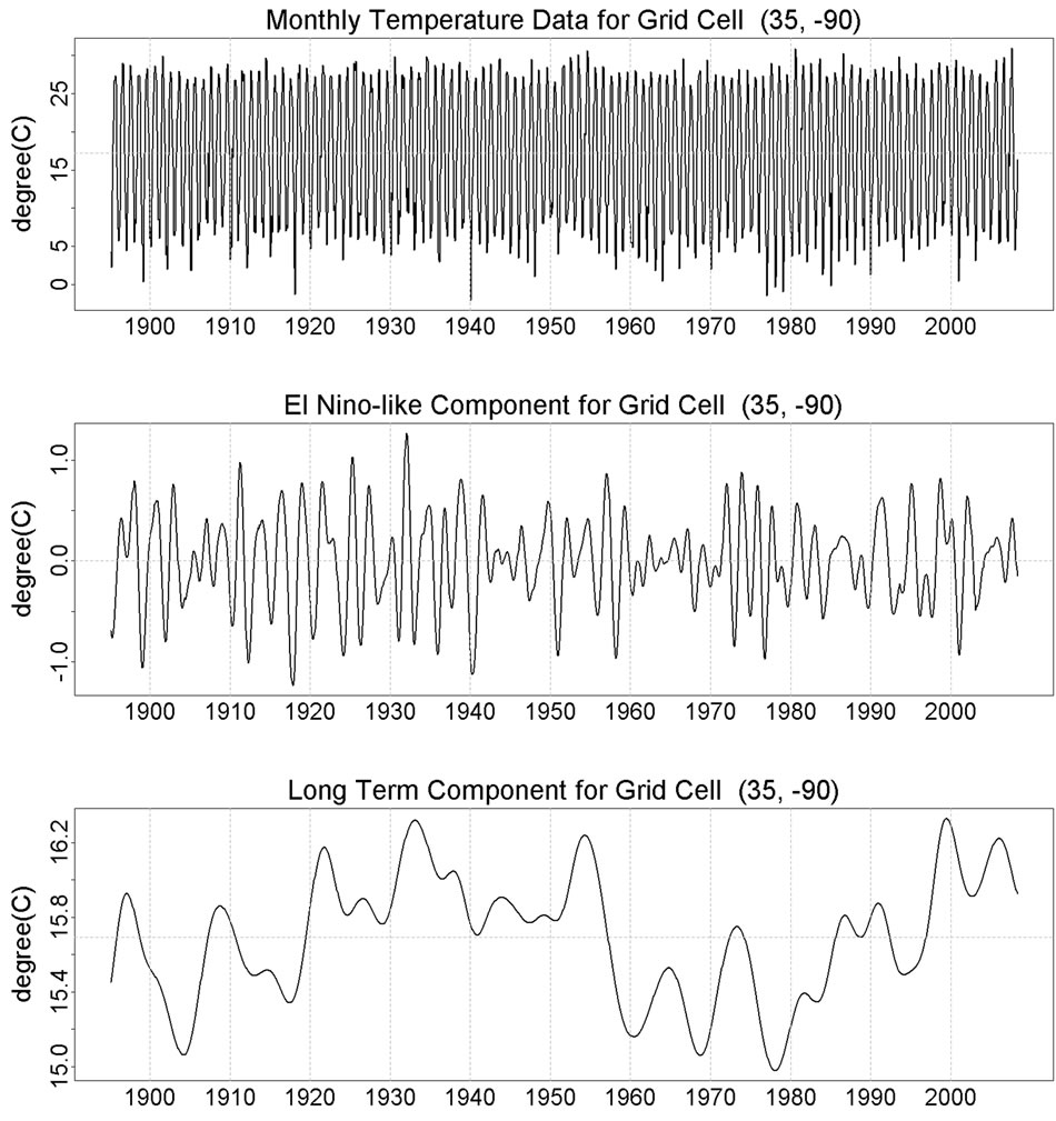
Figure 2. Tim series plots for raw data and decomposed components at grid cell (35, −90).
term component is spatially smoothed; its mean value is slightly different from the mean of raw data.
The spatial autocorrelation plot in Figure 3 reveals the spatial dependency for El Niño-like signal. The average correlation coefficients are higher than 0.5 when the distances of two location pairs are less than 1180 km. When the distance increases to 1850 km, the average correlation is still above 0.25. This result is consistent with Hansen’s work about temperature anomaly [5], and is much larger than the support range of KZ filters used for spatial smoothing. Theoretically, the critical range of KZ filter for spatial smoothing is only 750 km [15,26]; Our simulation shows that, for a Gaussian random field smoothed by KZ filters with the setting in Equations (6) and (7), the correlation coefficient is about 0.38 around 450 km, and only 0.24 around 555 km. The spatial dependency for El Niño-like signal is two times stronger than those of random fields. This result clearly suggests that the dependency comes from the component itself instead of KZ filters.
3.2. Global Long Term Component
Figure 4 exhibits the global long-term component after the latitude pattern and altitude effects are removed. The most apparent feature of Figure 4 is the regions with red color. The first is on the North Atlantic Ocean near the Northern Europe and Iceland, and its long-term mean temperature is 5˚C to 10˚C higher than other areas’ on the same latitude. The second area with red color is along 23.5˚ latitude, from northwestern India to Saudi Arabia

Figure 3. Average spatial correlation for El Niño components based on 10,000 samplings.
and Sarhra Desert—for most places in this region, their average temperatures are more than 5˚C higher compared with other areas’ on the same latitude; Southwestern USA (Arizona, etc.), and the Pacific coast of Canada and Alaska, also have warmer climates compared with other comparable regions; Part of Namibia and Botswana, some inland area of Australia also show similar “desert-like” climate pattern.
It is interesting to notice that these “hot spots” in middle and low latitude areas are consist with the annual global distribution of solar radiation [27], and their spatial distribution could be explained by the global surface and upper air circulation patterns. While in high latitude regions, the temperature difference could be explained by the effects of ocean currents.
The global long-term component also changed with time. Comparing Figure 5 with Figure 4, we can see that for most areas of the world, climate in early 1970s is cooler than climate of 2000s. This is consistent with the CET long-term component (see Figure 3 in [17]), in which the climate curve passed through a “valley” with relative low temperatures around 1970s, and 2000s is on the “mountain top” with the highest temperatures.
3.3. El Niño-Like Oscillations
El Nino-like oscillations is organized out of 2 - 5 years fluctuation and larger than 1200 km in geographical scale. Usually the magnitude of El Niño-like signal is smaller than the global long-term trend, but it changes much faster. The spatial patterns of El Niño-like signal are also more complex and keep changing with time. It is common that the El Niño-like variation in high latitude area is larger than that in tropical regions.
As an example, Figure 6 shows that Europe was in “deep blue” in the winter of 1941—the average temperature of this region was lower than the normal for 1.5˚C to 3˚C. It was this unusual bitter cold winter helped Russia in World War II. Another example is the Great Mississippi and Missouri Rivers Flood of 1993. As in Figure 7, most area of USA experienced cold climate in the spring
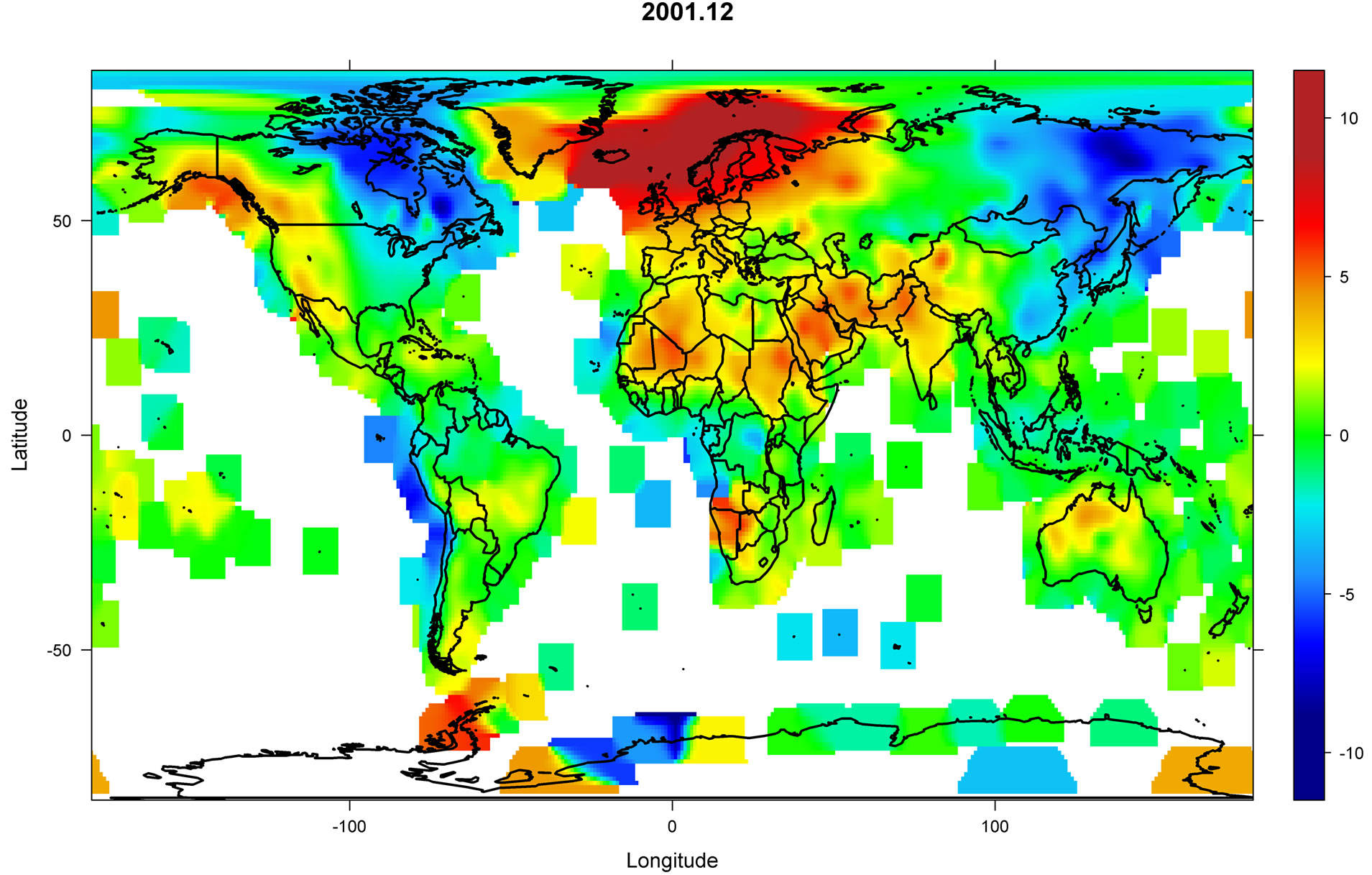
Figure 4. Global long-term component on December 2001. KZ filter m = (3˚, 3˚, 25 months), k = 5, adjusted for latitude and altitude effects.
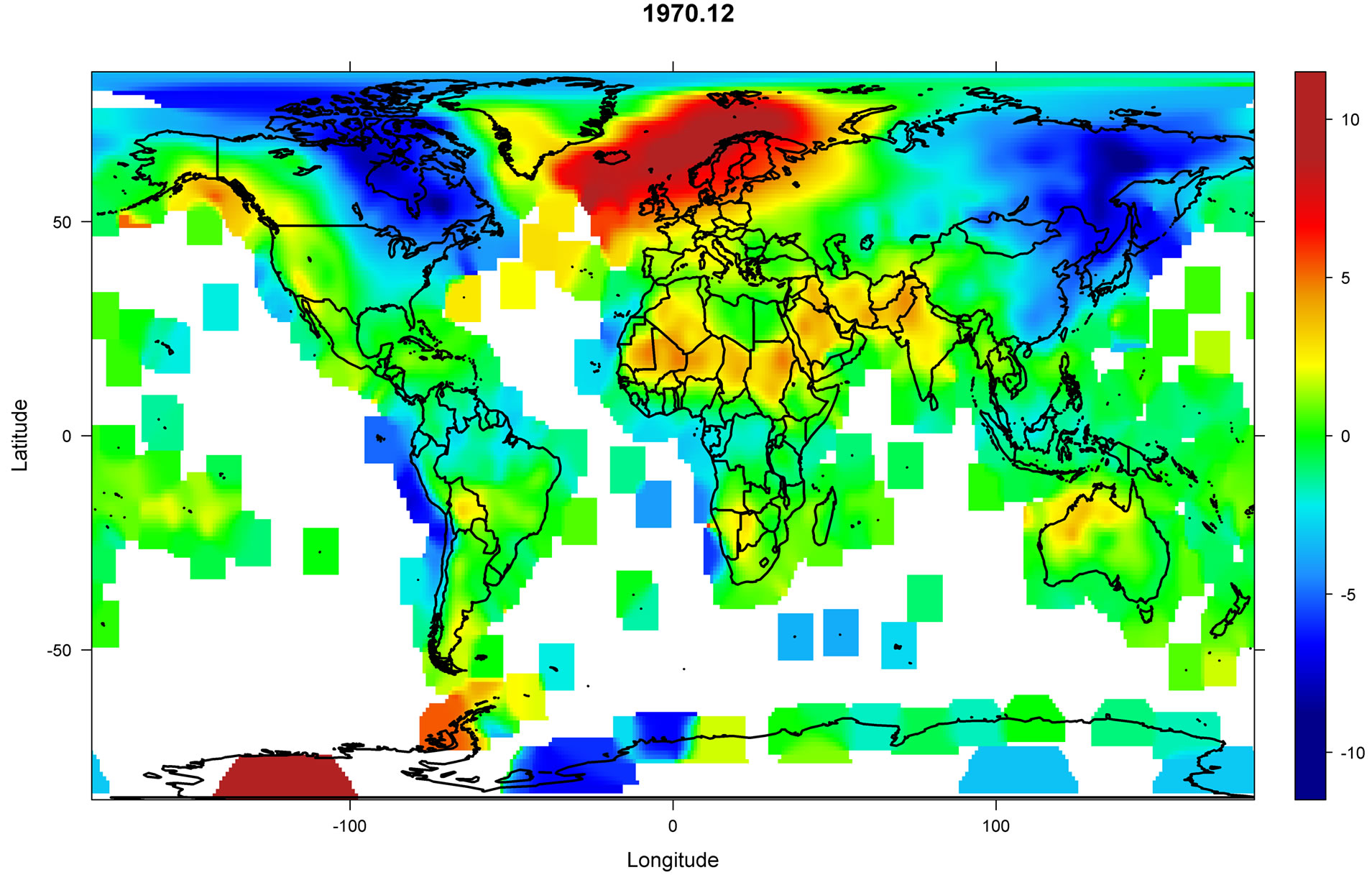
Figure 5. Global long-term component on December 1970. KZ filter m = (3˚, 3˚, 25 months), k = 5, adjusted for latitude and altitude effects.
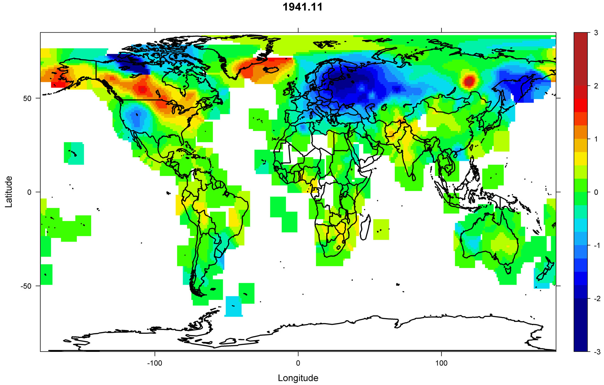
Figure 6. El Niño-like component—the cold climate of 1941 winter in Europe.

Figure 7. El Niño-like component—temperature dropped for most area of USA on April 1993. There was indication of very wet conditions at Midwestern USA at that period.
and summer of 1993; the blue color pervaded all Mississippi rive region. Zurbenko and Cyr had tried to connect this kind of temperature drops in large scale to big precipitation anomaly and intensive cloudy weather in the history of USA [17]. The serious drought in 2001 to 2002 can also be attributed to temperature anomaly caused by El Niño-like oscillations and global long-term trend. In the Eastern USA, the serious drought could be connected to the unusual high temperatures in the winter of 2001 to 2002 (Figure 8); while in the Western USA, the drought could be explained by the increased long-term temperature in this region (Figure 4).
Movies contain all history of Global and El Niño-like fluctuations in space and time for last 100 years can be provided separately from manuscript of the paper. Many slides out of it have been provided in the text.
4. Discussion
We had described the methodology to generate the global long-term temperature trend and El Niño-like oscillations from a seasonal changed raw temperature dataset. The annual seasonal change usually contains 90% energy of the variation. Specially designed KZ filters enabled us reconstruct the desired signals from background with high noise. The setting of KZ filter parameters has been confirmed by the spectral analysis and correlation analysis on their outputs.
Global long term component is recovering long term changes in spatial patterns of temperature. Zurbenko and Cyr [17] argued that part of those have been imposed partially by changing Sun activity, rest by human activity. Paper [28] is trying to partially explain periodic changes in Sun activity. El Niño-like scale perhaps is relevant to redistribution of energies over surface of the earth due to atmospheric and oceanic activities. Those two scales are different in their original nature and should not be kept together. Combination of them provides strong variability [29] and may start to confuse each other.
To generate the global long term component, the lapse rate value and the way to control the latitude pattern are critical. In the sensitive analysis, we had set higher lapse rates, and some mountain areas like Ecuador and Altiplano Plateau appeared to be redder, but the change in the major pattern of the long-term maps was negligible. Consequently, we believe that our method to select lapse rate is reasonable and had been supported by the data. However, since some nonlinear factors like snow line levels weren’t considered in the analysis, the accuracy for some mountain areas still has improvement space.
Generally speaking, the global long term component evaluates very slowly over the time. Its spatial pattern is

Figure 8. El Niño-like component on December 2001. There was indication of extra dry period at Eastern USA in that period.
stable and can be explained from the energy balance perspective. Red color in long term movie represents extra energy inputs in related grid cells. For example, Northern European area is warm due to the heat that the North Atlantic Current absorbed from southern ocean and carried to this area; so does the pacific coast of Canada and Alaska. Mean while, the surplus energy for Sahara and Arizona area comes from the extra solar irradiation associated with extreme low humidity and precipitation, low cloud coverage, or high altitudes and other local conditions. The maps of the long-term component could be a tool for predicting the general climate change trend of each region.
Spatial construction of filters provides outcomes from different data support on distance more than 500 km (smoothing scale of the filter). The spatial images are very well organized on much larger scales corresponding to the support regions for El Niño-like and long term scales that we are investigating. The El Niño movie captured some interesting phenomena of inter-annual climate change. Visual El Niño-like scales are of order more than 1000 km to 2000 km. We also observed temperature correlations on scale larger than our smoothing scale. Evidence from spectral analysis, correlation analysis and images displayed in our paper clearly support existence of such climate fluctuations in time and space.
El Niño-like fluctuations regularly last more than two years, and by KZ filter technology they may be predicted up to one year in advance everywhere over globe. This observation may provide us new inspiration to look into climate change study.
REFERENCES
- M. G. New, M. Hulme and P. D. Jones, “Representing Twentieth-Century Space-Time Climate Variability, Part I: Development of A 1961-1990 Mean Monthly Terrestrial Climatology,” Journal of Climate, Vol. 12, No. 3, 1999, pp. 829-856. doi:10.1175/1520-0442(1999)012<0829:RTCSTC>2.0.CO;2
- M. G. New, M. Hulme and P. D. Jones, “Representing Twentieth-Century Space-Time Climate Variability, Part II: Development of 1901-1996 Monthly Grids of Terrestrial Surface Climate,” Journal of Climate, Vol. 13, No. 13, 2000, pp. 2217-2238. doi:10.1175/1520-0442(2000)013<2217:RTCSTC>2.0.CO;2
- J. L. Caesar and R. Vose, “Large Scale Changes in Observed Daily Maximum and Minimum Temperatures: Creation and Analysis of a New Gridded Data Set,” Journal of Geophysical Research, Vol. 111, 2006, 10 p. doi:10.1029/2005JD006280
- J. H. Lawrimore, M. J. Menne, B. E. Gleason, C. N. Williams, D. B. Wuertz, R. S. Vose and J. Rennie, “An Overview of the Global Historical Climatology Network Monthly Mean Temperature Data Set, Version 3,” Journal of Geophysical Research, Vol. 116, No. D19121, 2011, 18 p. doi:10.1029/2011JD016187
- J. Hansen, R. Ruedy, M. Sato and K. Lo, “2010: Global Surface Temperature Change,” Reviews of Geophysics, Vol. 48, No. RG4004, 2010, 29 p. doi:10.1029/2010RG000345
- S. Solomon, et al., “Climate Change 2007: The Physical Science Basis, Contribution of Working Group I to the Fourth Assessment Report of the Intergovernmental Panel on Climate Change,” Cambridge University Press, New York, 2007.
- S. Huang, P. M. Rich, R. L. Crabtree, C. S. Potter and P. Fu, “Modeling Monthly Near-Surface Air Temperature from Solar Radiation and Lapse Rate: Application over Complex Terrain in Yellowstone National Park,” Physical Geography, Vol. 29, No. 2, 2008, pp. 158-178. doi:10.2747/0272-3646.29.2.158
- E. T. Linacre, “Climate Data & Resources,” Routledge, London, 1992.
- B. Finkenstadt, L. Held and V. Isham, “Statistical Methods for Spatio-Temporal Systems,” Chapman & Hall/ CRC, Boca Raton, 2007.
- E. Porcu, J. M. Montero and M. Schlather, “Advances and Challenges in Space-Time Modeling of Natural Events,” Springer-Verlag Berlin Heidelberg, New York, 2012. doi:10.1007/978-3-642-17086-7
- D. D. Cyr, “A Spline Kernel Based Smoothing Algorithm: A Comparison of Methods and a Spatiotemporal Application to Global Climate Fluctuations,” Ph.D. Thesis, State University of New York, Albany, 2010.
- K. G. Tsakiri and I. G. Zurbenko, “Prediction of Ozone Concentrations Using Atmospheric Variables,” Air Quality, Atmosphere & Health, Vol. 4, No. 2, 2011, pp. 111- 120. Hdoi:10.1007/s11869-010-0084-5
- S. T. Rao, I. G. Zurbenko, R. Neagu, P. S. Porter, J. Y. Ku and R. F. Henry, “Space and Time Scales in Ambient Ozone Data,” Bulletin of the American Meteorological Society, Vol. 78, No. 10, 1997, pp. 2153-2166. doi:10.1175/1520-0477(1997)078<2153:SATSIA>2.0.CO;2
- Organization for Economic Co-Operation and Development (OECD), “Section 4: Guidelines for the Reporting of Different Forms of Data,” In: Data and Metadata Reporting and Presentation Handbook, OECD Publishing, Paris, 2007, pp. 45-57.
- W. Yang and I. G. Zurbenko, “Kolmogorov-Zurbenko Filters,” Wiley Interdisciplinary Reviews: Computational Statistics, Vol. 2, No. 3, 2010, pp. 340-351. doi:10.1002/wics.71
- T. R. Karl, H. F. Diaz and G. Kukla, “Urbanization: Its Detection and Effect in the United States Climate Record,” Journal of Climate, Vol. 1, No. 11, 1988, pp. 1099- 1123. doi:10.1175/1520-0442(1988)001<1099:UIDAEI>2.0.CO;2
- I. Zurbenko and D. Cyr, “Climate Fluctuations in Time and Space,” Climate Research, Vol. 46, No. 1, 2011, pp. 67-76. doi:10.3354/cr00956
- P. E. Thornton, S. W. Running and M. A. White, “Generating Surfaces of Daily Meteorology Variables over Large Regions of Complex Terrain,” Journal of Hydrology, Vol. 190, No. 3, 1997, pp. 214-251.
- T. R. Blandford, K. S. Humes, B. J. Harshburger, B. C. Moore and V. P. Walden, “Seasonal and Synoptic Variations in Near-Surface Air Temperature Lapse Rates in a Mountainous Basin,” Journal of Applied Meteorology and Climatology, Vol. 47, No. 1, 2008, pp. 249-261. doi:10.1175/2007JAMC1565.1
- R. Dodson and D. Marks, “Daily Air Temperature Interpolated at High Spatial Resolution over A Large Mountainous Region,” Climate Research, Vol. 8, No. 1, 1997, pp. 1-20. Hdoi:10.3354/cr008001
- C. Rolland, “Spatial and Seasonal Variations of Air Temperature Lapse Rates in Alpine Regions,” Journal of Climate, Vol. 16, No. 7, 2003, pp. 1032-1046. Hdoi:10.1175/1520-0442(2003)016<1032:SASVOA>2.0.CO;2
- I. G. Zurbenko, S. T. Rao and R. Henry, “Mapping Ozone in the Eastern United States,” Environmental Manager, Vol. 1, No. 2, 1995, pp. 24-30.
- B. Close and I. Zurbenko, “KZA: Kolmogorov-Zurbenko Adaptive Filters,” R package, ver. 2.01, 2011.
- D. Cyr and I. Zurbenko, “Kzs: Kolmogorov-Zurbenko Spatial Smoothing and Applications,” R package, ver. 1.4, 2008.
- K. Stahl, R. D. Moore, J. A. Floyer, M. G. Asplin and I. G. McKendry, “Comparison of Approaches for Spatial Interpolation of Daily Air Temperature in a Large Region with Complex Topography and Highly Variable Station Density,” Agricultural and Forest Meteorology, Vol. 139, No. 3-4, 2006, pp. 224-236. Hdoi:10.1016/j.agrformet.2006.07.004
- I. G. Zurbenko, “The Spectral Analysis of Time Series,” North-Holland Series in Statistics and Probability, Elsevier, Amsterdam, 1986.
- W. D. Sellers, “Physical Climatology,” University of Chicago Press, Chicago, 1965. http://www4.uwsp.edu/geo/faculty/ritter/geog101/textbook/energy/global_patterns_of_heat_transfer.html
- I. Zurbenko and A. Potrzeba, “Tides in the Atmosphere,” Air Quality, Atmosphere and Health, 2011. Hdoi:10.1007/s11869-011-0143-6
- NASA/Goddard Space Flight Center, “Five-Year Average Global Temperature Anomalies from 1880 to 2010,” Scientific Visualization Studio. http://svs.gsfc.nasa.gov/vis/a000000/a003800/a003817
NOTES
*Corresponding author.