International Journal of Modern Nonlinear Theory and Application
Vol.04 No.04(2015), Article ID:61732,5 pages
10.4236/ijmnta.2015.44019
Dimension of Phase Point Trajectory
Kun Yao
Applied Physics Department, Naval University of Engineering, Wuhan, China

Copyright © 2015 by author and Scientific Research Publishing Inc.
This work is licensed under the Creative Commons Attribution International License (CC BY).
http://creativecommons.org/licenses/by/4.0/


Received 4 November 2015; accepted 4 December 2015; published 7 December 2015
ABSTRACT
In a physical system, phase point trajectory is impossible to be space-filling curve, of which the dimension is not greater than one. Equipotential map concept is proposed. When phase point trajectory dimension is 0, calculus tool is no longer applicable. System state can be changed instantly. When phase point trajectory dimension is 1, differential equation can be used to handle this case.
Keywords:
Trajectory, Dimension, System

1. Introduction
A system state is described by parameters. The choice of system parameters depends largely on our interests. A system phase space can be considered as a set of system parameters. A point in system phase space represents a system state, which is called phase point. For instance, if we care about the system hot and cold, then we will choose the temperature as the system parameter. The system phase space is temperature-line and continuous. For traffic light as a system, the color of which we care about, the system parameter is the noun describing the color. The system phase space is discrete and composed of three terms which are red, green and yellow. The presupposition that differential equation can be used to describe a system motion is that the system parameter varies continuously as time goes on. In this case, the phase point trajectory in phase space is a curve and continuous, of which the dimension is one. When the phase space is discrete, the calculus tools are no longer valid. In this case, the phase point trajectory is discrete, of which the dimension is zero.
Dimension is used to describe space characteristics of a set. Measure can indicate the size of space with the same dimension. For 1D space length indicates the size; for 2D space square indicates the size; for 3D space length cube indicates the size. Following this analogy, for n-D space length n-th power indicates the size. Dimension can be integer or fraction in accordance with different definitions. In vector space dimension is defined as a maximum number of linear independent vectors. In topology space, topology dimension is invariant in homeomorphic transformation. Ind, ind, dim are three commonly used definitions of topology dimension, which are equivalent in separable metric space. In accordance to the definition of topology dimension, its value is integer. The topology dimension of an empty set is −1, and a non-connected space is 0. The space characteristics distinguished by topology dimension are very coarse. There can be a great difference in the space characteristics of sets with the same topology dimension. A simple and famous example is the cantor set. Obviously the topology dimension of cantor set is 0. On the other hand, the cantor set dimension is ln2/ln3 calculated by the definition of Hausdorff dimension. Intuitively the cantor set is larger than an ordinary discrete set (its topology dimension is 0), and is less than a line (its topology dimension is 1). The space characteristic of such sets is called fractal. Hausdorff dimension is a finer definition than topology dimension. Finer geometry structure can be distinguished by Hausdorff dimension. Compared to ordinary graphics, the most important feature of fractal graphics is that we never draw a complete graph. We can approach to a fractal graph infinitely, but never reach it.
2. Phase Point Trajectory
A phase point trajectory of the physical system in phase space can be seen as a function of a one-dimensional timeline mapped to an m-dimensional manifold. M-dimensional manifold is determined by the constraints of the system. Each coordinate axis in phase space corresponds to a system parameter, and these parameters are used to describe the characteristics of the system. Once the parameters are given, a state of the system is determined. In classical mechanics, a point on the timeline corresponds to a point on phase point trajectory, and the system at a time point corresponds to only one state. In this case, the points on the time axis and the points on the trajectory are one to one mapping. Phase point trajectory of periodic motion is a closed curve. Its topological dimension is one. Ergodic motion phase point trajectory is a non-closed curve. Its topological dimension is a one. The curve is dense on m-dimensional manifold. In the strict sense, ergodic doesn’t mean that all the possible states of the system are experienced. Instead it means that any system status can be infinitely close in. The dimensions appeared in the rest of this article are topological dimensions.
Space-filling curve is a map from one-dimensional curve segment to a higher-dimensional space, such as well-known Peano curve, Hilbert curve, etc. These curves are the mappings of the one-dimensional line to two- dimensional plane. It can be seen from Net to theorem, if there is a bijective map between two manifolds with different dimensions, the map is necessarily discontinuous. Space-filling curve like Hilbert curve is not a bijective map. In the example of Hilbert curve, multiple points on the one-dimensional line segment are mapped to the same point on the square. There is one-to-one mapping of each point on the line segment to the square. Obviously such a mapping is discontinuous.
Here a simple example is considered. A particle moves in a line segment ab, and subject to the external force F(t). When the particle moves to the boundary of a and b point, Particle velocity value is constant, and the direction is reversed. This system phase space is two-dimensional as shown in Figure 1. The horizontal axis represents the spatial position of the particle. The vertical axis represents particle velocity. Phase point trajectory is assumed to be a space-filling curve. The curve covering the two-dimensional area is denoted by s. To make a line perpendicular to the x-axis x = x0, a < x0 < b. The intersection of the line and s is a line segment cd. Phase point trajectory and line cd intersect at a point when the trajectory passes through x = x0. Based on the assumption
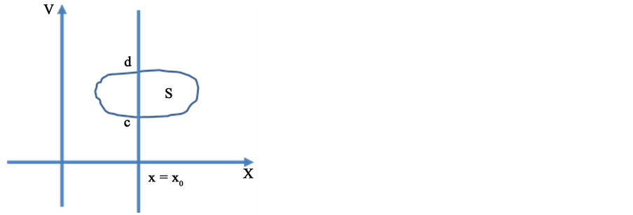
Figure 1. Particle phase space.
the trajectory can pass through every point on line cd. The number of times trajectory passes through x = x0 is countable, and the number of points on cd is discountable, which conflicts with each other. So phase point trajectory dimension in the system cannot be greater than 1.
The number of times that Phase point trajectory passes through a particular region in the phase space is countable. So for phase point trajectory in higher dimensional phase space, its dimension is impossible to be greater than one either. In classical mechanics systems, an interval on the timeline can be one to one mapped to the points in phase space. A phase point corresponds to a system state. The number of system states is discountable, and the dimension of phase point trajectory is one.
A system is considered, in which the number of states is infinite countable. System states are represented by natural numbers 1, 2, 3…. Beyond classical mechanics, consider a time point corresponds to an element in the power set of natural numbers. In other words, the system is in the case of multi-state superposition at a time point. A phase point represents a system superposition state. The power set of natural number and real number set are equipotential, so system superposition state can be one-to-one mapped on time line. The time sequence of phase points is determined by initial conditions and physical laws. In classical mechanics, a physical quantity used to describe a system is continuous. The value of a physical quantity corresponds to points on the real axis. So the values of physical quantity can be represented by real numbers and are arranged sequentially in ascending order on the real axis. The use of differential equations to describe the physical laws is based on the assumption that physical quantity changes continuously with time. For example, the system temperature is set increasing from T1 to T2. In this process system must be through all the temperature values between T1 and T2. This process of temperature change corresponds to a period of time.
When the number of system phase points is countable, phase point trajectory will be discontinuous. Trajectory is the jumping between different phase points. In this case, phase point trajectory is discrete, of which the dimension is 0. The change of system state cannot require a period of time but an instant. Considering a simple case, a system is assumed to have A, B, C three states, time period [t1, t2) corresponds to the state A, time period [t2, t3) corresponds to the state B, time period [t3, t4) corresponds to the state C. The time that these two processes of A to B and B to C take is 0. The process of A to C takes time t4 − t1. According to the view point of set theory, if the potential of phase point set is less than the potential of time set, the phase point trajectory is discontinuous. The system state can be changed instantly, which can be extended to the general case. If the potential of set A is greater than that of B, the mapping of A to B is discontinuous. A well-known example is the logistic equation [1]
 (1)
(1)
There is a real parameter k in this equation. Each k corresponds to the number of attractors. The number of attractors is a countable set. As the value of k changes continuously, the number of attractors will change suddenly. A k value regime [kn, kn + 1] corresponds to a bifurcation. Feigenbaum found such a law
 (2)
(2)
where  is a constant. Using this constant can roughly predict when the bifurcation occurs with the change of k. The period-doubling bifurcation phenomenon of other dynamic systems, also complies with the law described by Feigenbaum constant. This phenomenon will be extended to the general case which can be viewed as a mapping of a line of length L to the set of natural numbers. The line shown in Figure 2 is divided into n parts,
 . The length of each segment can be written in the form of series:
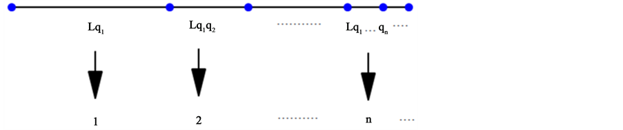
Figure 2. Map of line to natural numbers.
 (3)
(3)
 (4)
(4)
Each line segment corresponds to a natural number , where
 ,
,
 (5)
(5)
When the limit of qi is δ, it corresponds to double period bifurcations of dynamical system. Different qi limit corresponds to different bifurcation phenomenon.
All curves consist of a set, of which the potential is greater than that of the real number set. For the set composed of all curves, curves can be classified by equivalence classes. Each equivalence class of curves corresponds to a subset A. It is clear that all the curves equivalence classes are countable. A curve equivalence class corresponds to a system mode. There are different characteristics between the two modes of system. System mode can be defined according to different needs. In a differential dynamic system, different parameter values of differential equation correspond to different solutions. The solutions can be seen as a mapping of parameter range space to the curves. The potential of parameter range set is greater than the potential of the set composed of curve equivalence classes. When the parameter value changes continuously, the corresponding curve equivalence class may change. System mode conversion occurs. In weather forecast system, characteristic mode can be divided into sunny, cloudy, and rainy. Any solution of the weather system corresponds to a system mode. The phase point set can be represented by three points. In the Tokamak plasma experiments, phenomenon of spontaneous conversion between L mode and H mode is observed [2] . We can think of the plasma system parameters vary continuously. Phase point trajectory corresponds to two curve equivalence classes, in which one is L mode and the other one is H mode. Therefore when the plasma parameters change continuously, there can be a sudden change in plasma transport mode. There are two attractors in the well-known Lorentz model. With the continuous change of initial conditions, phase point will jump from one attractor to another attractor. Such sudden change of the system mode, which is due to the mapping of continuously varying parameter values are to countable system mode.
There may be such a dynamic system, of which the state is constantly changing. Assuming that a system has two states A, B, a function is defined similarly to Dirichlet function,

where t is time variable. If the variation law of the system state is described by this function, the system state will switch back and forth between A and B. The number that state A appears is countable. The number that state B appears is uncountable. Rational numbers, and irrational numbers are dense in the number axis. A and B are not adjacent. Supposing the system is in state A at time t0. We can confirm the system state at t0 + dt time, in the real physical world. dt depends on the accuracy of our instruments. In the actual measurement of time we generally get rational number, because we cannot finish a complete irrational number. If t0 + dt is rational, then the system is observed to be in state A. The actual measured time is rational. Rational numbers corresponding to state A is consistent with the actual law. If t0 + dt is irrational then observed that the system is in state B. But actually t + t0 we get is a rational number. We cannot prove experimentally that the system is in state B at the time of irrational numbers. Of course we can get a time point of irrational numbers. A particle oscillation period is assumed to be T, which is an irrational number by theoretical derivation. Time points of irrational number nT (n = 1, 2, ×××) can be obtained.
3. Discussions
f is assumed as a mapping of set A to set B. If A and B are equipotential then f is called equipotential map. If Aleph numbers of A and B are both 1, the map f can be described by differential equations. Dimension of phase point trajectory depends on the Aleph number of the set composed of system states. When the Aleph number of phase point set is equal to 0, the dimension of phase point trajectory is 0. Phase point trajectory is non-equipo- tential map. In this case, powerful differential equation is no longer valid. This is why the phenomenon of chaos is difficult to deal with. When the Aleph number of phase point set is equal to 1, the dimension of phase point trajectory is 1. Calculus tools can be used to handle this case. In the N-body problem the existence of non-colli- sion singularity has been proved [3] . System motion is unbounded within a limited time, of which the essence is that finite and infinite line can be one to one correspondence. In the limited time the length of phase point trajectory is infinite. In classical mechanics this mapping is allowed to exist, and material velocity is not limited. With regard to the special relativity theory, this mapping is not allowed to exist. Material velocity is limited.
Cite this paper
Kun Yao, (2015) Dimension of Phase Point Trajectory. International Journal of Modern Nonlinear Theory and Application,04,249-253. doi: 10.4236/ijmnta.2015.44019
References
- 1. May, R.M. (1976) Simple Mathematical Models with Very Complicated Dynamics. Nature, 261, 459-467.
http://dx.doi.org/10.1038/261459a0 - 2. Connor, J.W. and Wilson, H.R. (2000) A Review of Theories of the L-H Transition. Plasma Physics and Controlled Fusion, 42, R1.
http://dx.doi.org/10.1088/0741-3335/42/1/201 - 3. Xia, Z. (1992) The Existence of Noncollision Singularities in Newtonian Systems. Annals of Mathematics, 135, 411-468.
http://dx.doi.org/10.2307/2946572