Open Journal of Fluid Dynamics
Vol.05 No.04(2015), Article ID:62026,11 pages
10.4236/ojfd.2015.54032
Nonlinear Vortex Structures in Obliquely Rotating Fluid
Michael Kopp1,2, Anatoly Tur3, Vladimir Yanovsky1,2
1Institute for Single Crystals, National Academy of Sciences of Ukraine, Kharkov, Ukraine
2V.N. Karazin Kharkiv National University 4 Svobody Sq., Kharkov, Ukraine
3Université de Toulouse [UPS], CNRS, Institut de Recherche en Astrophysique et Planétologie, Toulouse Cedex, France

Copyright © 2015 by authors and Scientific Research Publishing Inc.
This work is licensed under the Creative Commons Attribution International License (CC BY).


Received 22 September 2015; accepted 14 December 2015; published 18 December 2015

ABSTRACT
In this paper, we find a new large scale instability which appears in obliquely rotating flow with the small scale turbulence, generated by external force with small Reynolds number. The external force has no helicity. The theory is based on the rigorous method of multi-scale asymptotic expansion. Nonlinear equations for instability are obtained in the third order of the perturbation theory. In this article, we explain in detail the nonlinear stage of the instability and we find the nonlinear periodic vortices and the vortex kinks of Beltrami type.
Keywords:
Large Scale Vortex Instability, Coriolis Force, Multi-Scale Asymptotic Development, Small Scale Turbulence, Vortex Kinks

1. Introduction
It is well known that the rotating effects play an important role in many theoretical and practical applications for fluid mechanics [1] and are especially important for geophysics and astrophysics [2] -[4] when one has to deal with rotating objects such as the Earth, Jupiter, the Sun, etc. Rotating fluids could generate different wave and vortex motions, for example, gyroscopic waves, Rossbywaves, internal waves, located vortices and coherent vortex structures [4] - [7] . Among the vortex structures, the most interesting are the large scale ones since they carry out the efficient transport of energy and impulse. The structures which have characteristic scale much more than the scale of turbulence or the scale of external force which generates this turbulence are understood as large scale ones. In this paper we find a new large scale instability in obliquely rotating flow which is influenced by the small scale external force with zero helicity. Its axis of rotation does not coincide with the Z axis. This force supports small scale turbulent fluctuations in fluid. The nonlinear large scale helical vortex structures such as Beltrami vortices or localized kinks appear as a result of the development of this instability in rotating fluid. This supposes that the external mall-scale force substitutes the action of small-scale turbulence. Further we consider that the external force acts in the plane (X, Y). Instability occurs only when the vector of angular velocity of rotation  is inclined relatively to the plane (X, Y), as shown in Figure 1. If the fluid is rotating around the axis Z strictly, then instability does not occur. The helical 2D velocity field
  turns around the axis Z when Z changes in the periodic wave (Figure 2) and makes one turn in the kink (Figure 3). The found instability belongs to the class of instabilities called hydrodynamic α-effects. For these instabilities the positive feedback between velocity components is typical:
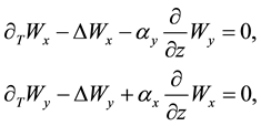

Figure 1. In general, the angular velocity Ω is inclined relatively to the plane (X, Y) in which there is an external force .
.

Figure 2. Nonlinear helical Beltramiwave, which corresponds to the closed trajectory in the phase plane ( ,
, ). The spiral is oriented along Z axis and inclined relatively to the axis of rotation.

Figure 3. Localized solution (kink), which corresponds to the separatrice in the phase plane ( ,
, ).
).
and leads to the instability. α-effect origins from magnetic hydrodynamics where it engenders the increase of large scale magnetic fields (see for example, [8] ). Later it was extended to ordinary hydrodynamics. Several examples of hydrodynamics α-effect [9] - [16] are known for today. From this point of view, in this study we found a new example of the α-effect. The theory of this instability is based on a rigorous method of multi-scale development, which was proposed by Frisch, She and Sulem for the theory of the AKA effect [14] . This method allows finding the equations for large scale perturbations in the form of secular equations of the asymptotic theory, to calculate the Reynolds stress tensor and to find the instabilities. The small parameter of asymptotical development is the number of Reynolds  Our paper is organized as follows: in Section 2 we formulate the problem and the main equations in rotating system coordinates; in Section 3 we discuss the concept of multi-scale development and we give the secular equations. In Section 4 we calculate the velocity field of zero approximation. In Section 5 we describe the calculation of the Reynolds stress and find the large scale instability. In Section 6 we discuss the saturation of the instability and find the nonlinear stationary vortex structures. The results obtained are discussed in the conclusions given in Section 7.
2. The Main Equations and Formulation of the Problem
Let us examine the equations of motion for non-compressible rotating fluid with the external force  in rotating coordinates system:
 (1)
(1)
 (2)
(2)
The external force  is divergence-free. Here
  is angular velocity of fluid rotation,
  is viscosity and
  is constant fluid density. Let us designate the characteristic amplitude of force as f0, and its characteristic space and time scale as λ0 and t0 respectively.
Then . We will designate the characteristic amplitude of velocity, generated by external
force as v0. Further we choose the dimensionless variables :
:


Then, in dimensionless variables the equation (1) takes the form:
 (3)
(3)
 . Where R and
  are respectively the Reynolds number and the Taylor
number on scale . Further we will consider the Reynolds number as small
  and will construct on this small parameter the asymptotical development. Concerning the parameter D, we do not choose any range of values for the moment. Let us examine the following formulation of the problem. We consider the external force as being of small scale and of high frequency. This force leads to small scale fluctuations in velocity. After averaging, these rapidly oscillating fluctuations vanish. Nevertheless, due to small nonlinear interactions in some orders of perturbation theory, nonzero terms can occur after averaging. This means that they are not oscillatory, that is to say, they are large scale. From a formal point of view, these terms are secular, i.e., they create the conditions for the solvability of large-scale asymptotic development. So, the purpose of this paper is to find and study the solvability equations, i.e., the equations for the large scale perturbations. Let us denote the small scale variables by
 , and the large scale ones by
 . The small scale partial derivative operation
 , and the large scale ones
  are written, respectively, as
  and
and . To construct a multi-scale asymptotic development we follow the method which is proposed in [8] .
3. The Multi-Scale Asymptotic Development
Let us search the solution to equations (2) and (3) in following form:
 (4)
(4)
 (5)
(5)
We introduce the slow variables  and
and  which lead to the following expressions for the spatial and temporal derivatives:
 (6)
(6)
 (7)
(7)
 (8)
(8)
Using initial notation, the system of equations can be written as:
 (9)
(9)
 (10)
(10)
Substituting these expressions into the initial equations (2) and (3) and then gathering together the terms of the same order, we obtain the equations of the multi-scale asymptotic development and write down the obtained equations up to order  including. In the order
  there is only one equation:
 (11)
(11)
In order  we have the equation:
 (12)
(12)
In order  we get a system of equations:
 (13)
(13)
 (14)
(14)
The system of equations (13) and (14) gives secular terms
 (15)
(15)
which corresponds to a geostrophic equilibrium equation. In zero order , we have the following system of equations:
 (16)
(16)
 (17)
(17)
These equations give the following secular equation:
 (18)
(18)
Let us consider the equations of the first approximation R:
 (19)
(19)
 (20)
(20)
Secular equations follow from this system of equations:
 (21)
(21)
 (22)
(22)
Secular equations (21) and (22) are satisfied by choosing the following geometry for the velocity field (Beltrami field):
 (23)
(23)

In the second order , we obtain the equations:
 (24)
(24)
 (25)
(25)
It is easy to see that there are no secular terms in this order.
Let us come now to the most important order . In this order we obtain the equations:
 (26)
(26)

From this we get the main secular equation:
 (27)
(27)
There is also an equation to find the pressure :
:
 (28)
(28)
4. The Velocity Field in Zero Approximation
It is clear that the most important is the equation (27). In order to obtain these equations in closed form, we need to calculate the Reynolds stress . First of all, we have to calculate the fields of the zero approximation
 . From the asymptotic development in zero order we have:
 (29)
(29)
Let us introduce the operator :
:
 (30)
(30)
Using , we rewrite equation (29) in the form:
 (31)
(31)
Pressure P0 can be found from condition 
 (32)
(32)
Let us introduce the designations for the operators:
 (33)
(33)
and for velocities:  Then excluding pressure from (31), we obtain the system of equations to find the velocity field of zero approximation:
 (34)
(34)
In order to solve this system of equations we have to set the force in the explicit form. Let us choose now the external force in the rotating system of coordinates in the following form:

It is obvious that divergence and helicity of this force us equal to zero:  Thus, the external force is given in the plane (x, y), which is orthogonal to the projection of angular velocity
 .
.
The solution for equations system (34) can be found easily in accordance with Cramer’s Rule:
 (35)
(35)
Here  is the determinant of the system (34):
 (36)
(36)
 (37)
(37)
 (38)
(38)
 (39)
(39)
Expanding the determinant, we obtain:
 (40)
(40)
 (41)
(41)
 (42)
(42)
 (43)
(43)
In order to calculate the expressions (40)-(43) we present the external force in complex form:
 (44)
(44)
Then all operators in formulae (40) - (42) act from the left on their eigenfunction. In particular:
 (45)
(45)
To simplify the formulae, let us choose 
Now let us designate:
 (46)
(46)
Before doing further calculations, we have to note that some components of tensors  and
and  vanish. Let us write the non-zero components only:
 (47)
(47)
Taking into account the formulae (45)-(47), we can find the determinant:
 (48)
(48)
In a similar way we find velocity field of zero approximation:
 (49)
(49)
 (50)
(50)
 (51)
(51)
We note that the angular velocity  component disappears from the expression for the velocity field of zero approximation, which is a consequence of the properties of an external force.
5. Reynolds Stress and Large Scale Instability
To close the equations (27) we have to calculate the Reynolds stresses  and
and . These terms are easily calculated with the help of formulae (49)-(51). As a result we obtain:
 (52)
(52)
Now equations (27) are closed and take form:
 (53)
(53)
We calculate the modules and write the equations (53) in the explicit form:
 (54)
(54)
With small  we obtain the linearized equations (54):
 (55)
(55)

The system (55) describes the positive feedback between the components of velocity. We will look for the solution of linear system (55) in the following form:
 (56)
(56)
Substituting (56) in equation (55), we obtain the dispersion equation:
 (57)
(57)
The dispersion equation (57) shows the existence at  of the large scale instability with maximum
growth rate  at the wave vector
  As a result of the development of instability
the large scale helical Beltrami vortices are generated in the system. When , damped oscillations with
a frequency  arise instead of instability. In fact the behavior of
  depends on how is located the
external force  with respect to the perpendicular projections of the angular velocity of rotation and the values of components
  If one of the component
  is zero or equals to
 , then the instability is absent. Instability exists in the following cases:

In all other cases damped oscillations occur.
6. Saturation of Instability and Nonlinear Vortex Structures
It is clear that with increasing of amplitude nonlinear terms decrease and instability becomes saturated. Consequently stationary nonlinear vortex structures are formed. To find these structures let us choose equations (54)
 and integrate equations one time over Z. We obtain the system of equations:
 (58)
(58)
Let’s take for this system new variables:  Then we obtain:
 (59)
(59)
The system of equations (59) can be written in Hamiltonian form:

Where Hamiltonian H has the form:
 (60)
(60)
with function :
:
 (61)
(61)
Integral in expression (61) is calculated in elementary functions [17] . Let us choose for simplicity  In this case, the function (61) is equal to [17] :
 (62)
(62)
The sum  can be written down as one formula. Then Hamiltonian is equal to:
 (63)
(63)
It is easy to construct the phase portrait of Figure 4 for Hamiltonian (63) and specific values ,
, . The phase portrait shows the presence of closed trajectories in the phase plane around elliptic points and separatrices that connect hyperbolic points. It is obvious that the closed trajectories correspond to nonlinear periodic solutions. The separatrices correspond to localized solutions of kink type.

Figure 4. Phase plane for Hamiltonian (63) ( ,
, ). We see the presence of closed trajectories around the elliptic points and separatrices which connect the hyperbolic points. Phase portrait is typical for Hamiltonian systems.
7. Conclusions and Discussion of the Results
In this work we found new large scale instability in rotating fluid. It is supposed that the small scale vortex external force in rotating coordinates system acts on fluid which maintains the small velocity field fluctuations (small-scale turbulence with low Reynolds number ). For the real applications this Reynolds number should be calculated with the help of the turbulent viscosity. The asymptotic development of motion equations by small Reynolds number allows obtaining motion equations for the large scale. These equations are of the hydrodynamic α-effect type, in which velocity components
  are connected by the positive feedback. This may result in the appearance of the large scale vortex instability. This instability is responsible for the formation of large scale Beltrami vortices in rotating fluid with small scale external force. With further increase of amplitude the instability stabilizes and passes to a stationary mode. In this mode the nonlinear stationary vortex structures are formed. The most interesting structures belong to a variety of vortex kinks. These kinks connect stationary hyperbolic points of the dynamical system (58).
Note that in contrast to previous work on the hydrodynamic α-effect in rotating fluid, the method enables us to construct an asymptotic development in a natural way and to explore non-linear theory of nonlinear stationary vortex kinks.
Cite this paper
MichaelKopp,AnatolyTur,VladimirYanovsky, (2015) Nonlinear Vortex Structures in Obliquely Rotating Fluid. Open Journal of Fluid Dynamics,05,311-321. doi: 10.4236/ojfd.2015.54032
References
- 1. Grinspen, H.P. (1990) The Theory of Rotating Fluids. Brookline Press, Brooklyn, MA.
- 2. Roberts P.H. and Soward, A.M., Eds. (1978) Rotating Fluids in Geophysics. Acad. Press Inc., London.
- 3. Clarke, C. and Carswell, B. (2007) Principles of Astrophysical Fluid Dynamics. Cambridge University Press, Cambridge, UK.
http://dx.doi.org/10.1017/CBO9780511813450 - 4. Vallis, G.K. (2010) Atmospheric and Oceanic Fluid Dynamics. Cambridge University Press, Cambridge, MA.
- 5. Abramowicz, M.A., Lanza, A., Spigel, E.A. and Szuszkiewicz, E. (1992) Vortices on Accretion Disks. Nature, 356, 41-43.
http://dx.doi.org/10.1038/356041a0 - 6. Brandt, P.N., Scharmer, G.B., Ferguson, S., Shine, R.A., Tarbell, T.D. and Title, A.M. (1988) Vortex Flow in the Solar Photosphere. Nature, 335, 238-240.
http://dx.doi.org/10.1038/335238a0 - 7. Dritschel, G. and Legras, B. (1993) Modeling Oceanic and Atmospheric Vortices. Physics Today, 46, 44.
http://dx.doi.org/10.1063/1.881375 - 8. Moffat, H.K. (1978) Magnetic Field Generation in Electrically Conducting Fluids. Cambridge University Press, Cambridge, UK.
- 9. Moiseev, S.S., Sagdeev, R.Z., Tur, A.B., Khomenko, G.A. and Yanovsky, V.V. (1983) Theory of Large-Scale Structures in Hydrodynamic Turbulence. ZHETF, 58, 1149.
- 10. Moiseev, S.S., Rutkiewicz, P.B., Tur, A.B. and Yanovsky, V.V. (1988) Spiral Vortex Dynamo in Turbulent Convection. ZHETF, 67, 294.
- 11. Loupian, E.A., Mazurov, A.A., Rutkiewicz, P.B. and Tur, A.B. (1992) Generation of Large-Scale Eddies as a Result of the Spiral Turbulence Convective Nature. ZHETF, 75, 833.
- 12. Khomenko, G.A., Moiseev, S.S. and Tur, A.V. (1991) The Hydrodynamic Alpha-Effect in a Compressible Fluid. Journal of Fluid Mechanics, 225, 355-369.
http://dx.doi.org/10.1017/S0022112091002082 - 13. Levina, G.V., Moiseev, S.S. and Rutkevich, P.B. (2000) Hydrodynamic Alpha-Effect in a Convective System. Advances in Fluid Mechanics, 25, 111-162.
- 14. Frisch, U., She, Z.S. and Sulem, P.L. (1987) Large-Scale Flow Driven by the Anisotropic Kinetic Alpha Effect. Physica D: Nonlinear Phenomena, 28, 382-392.
http://dx.doi.org/10.1016/0167-2789(87)90026-1 - 15. Tur, A.V. and Yanovsky, V.V. (2013) Non Linear Vortex Structures in Stratified Fluid Driven by Small-Scale Helical Force. Open Journal of Fluid Dynamics, 3, 64-74.
http://dx.doi.org/10.4236/ojfd.2013.32009 - 16. Kitchatinov, L.L., Rudiger, G. and Khomenko, G. (1994) Large-Scale Vortices in Rotating Stratified Disks. Astronomy and Astrophysics, 287, 320-324.
- 17. Gradshteyn, I.S. and Ryzhik, I.M. (1974) Tables of Integrals, Sums, Series and Products. Academic Press, San Diego, San Francisco, New York, Boston, London, Sydney, Tokyo.