Open Journal of Fluid Dynamics
Vol.4 No.1(2014), Article ID:44079,25 pages DOI:10.4236/ojfd.2014.41004
Sharpening Diffuse Interfaces with Compressible Flow Solvers
Nicolas Favrie1, Sergey Gavrilyuk1, Boniface Nkonga2, Richard Saurel1
1Aix-Marseille University, Marseille, France
2J.A. Dieudonné Mathematics Lab., University Nice-Sophia Antipolis, Nice, France
Email: nicolas.favrie@univ-amu.fr, sergey.gavrilyuk@univ-amu.fr, boniface.nkonga@unice.fr, richard.saurel@univ-amu.fr
Copyright © 2014 by authors and Scientific Research Publishing Inc.
This work is licensed under the Creative Commons Attribution International License (CC BY).
http://creativecommons.org/licenses/by/4.0/


Received 17 January 2014; revised 17 February 2014; accepted 24 February 2014
Abstract
Diffuse interfaces appear with any Eulerian discontinuity capturing compressible flow solver. When dealing with multifluid and multimaterial computations, interfaces smearing results in serious difficulties to fulfil contact conditions, as spurious oscillations appear. To circumvent these difficulties, several approaches have been proposed. One of them relies on multiphase flow modelling of the numerically diffused zone and is based on extended hyperbolic systems with stiff mechanical relaxation (Saurel and Abgrall, 1999 [4] , Saurel et al., 2009 [6] ). This approach is very robust, accurate and flexible in the sense that many physical effects can be included: surface tension, phase transition, elastic-plastic materials, detonations, granular effects etc. It is also able to deal with dynamic appearance of interfaces. However it suffers of an important drawback when long time evolution is under interest as the interface becomes more and more diffused. The present paper addresses this issue and provides an efficient way to sharpen interfaces. A sharpening flow model is used to correct the solution after each time step. The sharpening process is based on a hyperbolic equation that produces a steady shock in finite time at the interface location. This equation is embedded in a “sharpening multiphase model” redistributing volume fractions, masses, momentum and energy in a consistent way. The method is conservative with respect to the masses, mixture momentum and mixture energy. It results in diffused interfaces sharpened in one or two mesh points. The method is validated on test problems having exact solutions.
Keywords:Material Interfaces; Multifluid; Multiphase; Multimaterial; Shocks; Non-Conservative; Hyperbolic Equations

1. Introduction
Numerical smearing of interfaces (or contact discontinuities) appears with any Eulerian discontinuity capturing compressible flow solver. In the context of the Euler equations, it results in at least four points in the capturing zone and the number of points increases during time evolution with most methods. When dealing with multifluid and multimaterial computations, diffuse interfaces result in serious difficulties to match interface conditions, as spurious oscillations appear. To circumvent these difficulties, several approaches have been proposed.
Lagrangian methods and Front Tracking schemes are aimed to remove artificial smearing but result in other difficulties.
Interface reconstruction methods (Hirt and Nichols, 1981 [1] , Youngs, 1989 [2] ) are aimed to restore sharp interfaces with the help of a volume fraction reconstruction algorithm but do not consider mass, momentum and energy redistribution. Moreover, these methods are more suitable for non-compressible fluids.
Level-set methods (Fedkiw et al., 1999 [3] ) are now very popular as they result in sharp interface representation and are quite easy to implement. They present however robustness and conservation issues.
Another option relies on multiphase flow modelling of the numerically diffused zone and is based on extended hyperbolic systems with stiff relaxation (Saurel and Abgrall, 1999 [4] , Kapila et al., 2001 [5] , Saurel et al., 2009 [6] ). This approach is very robust, simple to implement, accurate and flexible in the sense that many physical effects can be included such as:
• surface tension (Perigaud and Saurel, 2005 [7] , Braconnier and Nkonga 2009 [8] )• phase transition fronts and cavitation (Saurel et al., 2008[9] )• solid materials (Favrie et al., 2009 [10] , Favrie and Gavrilyuk, 2012 [11] )• detonations waves in heterogeneous energetic materials (Petitpas et al., 2009 [12] )• powder compaction including gas permeation effects (Saurel et al., 2010 [13] ).
This method is also able to deal with dynamic interfaces appearance. However it suffers of an important drawback when long time evolutions are under interest as the interface becomes more and more diffused. This has been clearly understood by Kokh and Lagoutière (2010) [14] where an antidiffusion scheme is built. So et al. (2012) [15] presented another approach able to sharpen interfaces by removing the artificial viscosity excess present at contact discontinuities with Godunov type schemes. In this method the determination to the diffusion that should be removed is not straightforward.
The present paper addresses this issue with another way to sharpen interfaces. The artificial compression method of Harten (1977 [16] , 1978 [17] ) is revisited. The main idea with this method is to create an artificial shock at the interface during a correction step. A similar idea has been considered and adapted by Shukla et al. (2010) [18] to the context of a simplified diffuse interface model (Allaire et al., 2002 [19] , Massoni et al., 2002 [20] ). But in this paper the conservation of the mass is only guarantied at first order.
We continue this effort in the present paper by addressing:
• A more general diffuse interfaces flow model, where the physical effects previously mentioned can be considered, in particular dynamic interfaces creation.
• Mass, momentum and energy redistribution across the interface during the sharpening process. This issue has never been considered prior to the present work.
The present method uses an extra hyperbolic equation for a function that is equal to zero on one side of the interface and to one on the other side. Contrarily to Volume of Fluid, Level-set and multiphase flow models, this equation is not a transport one. It corresponds to a hyperbolic conservation law that admits shocks. More precisely, steady shocks appear at the location where this function is equal to 0.5. Thus, starting from a diffused solution, after for example one or several steps of the diffuse interface method, the volume fraction, density, energy fields are diffused. The volume fraction field is then sharpened with the help of the new function during a correction step. The main difficulty is to synchronise mass, momentum and energy sharpening with the volume fraction one. Also, this correction has to be conservative. Synchronisation of the various sharpening processes while maintaining conservation are the main goals and difficulties of the present work.
The resulting scheme is able to handle material interfaces in one or two mesh points. The single phase limit of the multiphase model and method corresponds to a scheme that improves the results of conventional capturing schemes used for the Euler equations.
The paper is organised as follows. In Section 2, the sharpening function is introduced with its evolution equation. Its ability to sharpen diffused profiles by the means of shock formation is demonstrated. In Section 3, the diffuse interface model of Saurel et al. (2009) [6] is recalled. This single velocity, pressure non-equilibrium model is solved in the limit of stiff pressure relaxation to solve the Kapila et al. (2001) [5] model. In Section 4, the interface sharpening method is presented. This correction step consists in synchronising the sharpening function process with repartition of mass, momentum and energy of the various phases while preserving conservation for the mixture. In Section 5, numerical approximation of the interface sharpening model is detailed. Computational examples, illustrations and validations are given in Section 6. Method’s extension to an arbitrary number of fluids is given in Section 7. Conclusions are given in Section 8.
2. Sharpening Function
Let’s consider two phases separated by an interface. The sharpening function  is used to detect the presence of phase 1. When the phase 1 is pure, then
  and
and . In mixture zones, or diffused interface zones,
 . The constraint
  holds everywhere.
Let’s consider a particular case of a mixture zone separating phase 1 on the right and phase 2 on the left, as shown in Figure 1.
In this particular situation where  the sharpening equation reads:
 (2.1)
(2.1)
where a is a positive arbitrary parameter that controls the rate at which sharpening occurs. This parameter is not describing any physical effects and this equation will be used only to sharpen interfaces. Since the sharpening parameter a is arbitrary, in the following we will pose , a pseudo time. Thus the previous equation reads:

As  it also reads,
 .
.
The characteristic slope is thus,
 .
.
This slope is positive if , and negative if
 .
.
Equation (2.1) admits shocks appearing in finite time. Consider a left state (L) and a right state (R) separated by a shock. The shock propagation speed  is given by:
 (2.2)
(2.2)
If , the Lax stability criterion is satisfied:
 .
.
The Riemann problem solution is schematized in the Figure 2.
For any point of the initial data corresponding to Figure 1, the Riemann problem solution thus reads:
 (2.3)
(2.3)
The Godunov method for equation (2.1) reads:
 (2.4)
(2.4)
This method is stable under the following CFL condition:
 ,
,
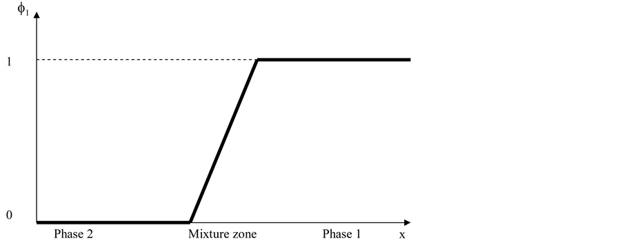
Figure 1. Schematic representation of a mixture zone separating two pure fluids, phase 1 on the right and phase 2 on the left.
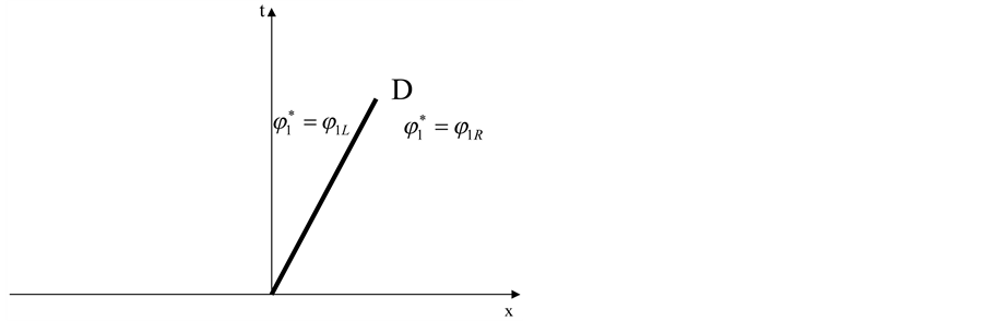
Figure 2. Schematic representation of the Riemann problem solution of Equation (II.1), valid when .
.
i.e.
 . (2.5)
Let’s examine the solution given by this method for the initial condition shown in the Figure 1. A 200 cells mesh is considered for a domain of 1 m length. The 30 first cells have  as initial data and the 30 last cells have
 . The mixture zone thus corresponds to 140 cells with a linear
  profile. The solution obtained with scheme (2.4) using (2.3) and (2.2) is shown at pseudo times
 ,
,  ,
,  and
and . The corresponding results are shown in Figure 3.
Equation (2.1) is however a simplified form of a more general equation, valid only if .
.
In one-dimension, we suppose here that the volume fraction regular enough i.e. two interfaces are not too close the general form of the sharpening equation is,
 . (2.6)
This is equivalent to (in the case of monotonic behaviour of ):
):
 .
.
In multi-dimensional case, it generalizes as:
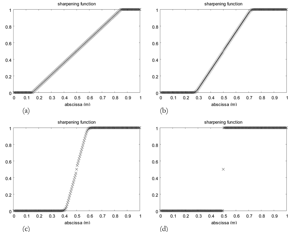
Figure 3. Numerical solution of Equation (2.1) with the Godunov method. The initial condition is shown in graph (a). The numerical solution is shown at pseudo time  on graph (b), at time
  on graph (c) and at final time (
 ) on graph (d). After this time, the solution remains unchanged. A sharp discontinuity appears from a diffuse zone.
 . (2.7)
The sharpening equation (2.6) or (2.7) is going to play a central role in the interface sharpening process. Indeed, the sharpening function  is not so far of the volume fraction
  used in multiphase flow modelling and in diffuse interface theory.
Before going on with the sharpening method, it is important to recall and summarize the basis of the diffuse interface method given in Saurel et al. (2009) [6] . The sharpening method will be used as a correction step in this frame. The diffuse interface step solves interface motion and wave’s dynamics with perfect fulfilment of interface conditions.
3. Diffuse Interface Method
The diffuse interface model under consideration is the one of Kapila et al. (2001) [5] . This system involves a nonconservative equation that results in numerical difficulties. A pressure non-equilibrium formulation was proposed in Saurel et al. (2009) [6] to solve this system with a sequence of three sub steps, each one being simple and robust. In this paper, we follow the Saurel et al. (2009) [6] approach to solve the “target system” of Kapila et al. (2001) [5] .
3.1. Target System
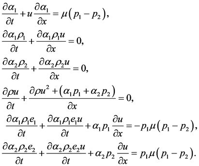
The Kapila et al. (2001) model in the context of two fluids reads:
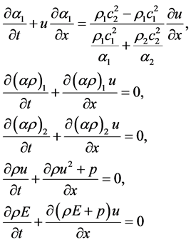 (3.1)
(3.1)
where , and e represent respectively the volume fraction, the mixture density, the velocity, the mixture pressure, the mixture total energy and the mixture internal energy.
The mixture internal energy is defined as,
 (3.2)
(3.2)
and the mass fractions are given by .
.
The mixture density is defined by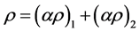 .
.
Each fluid is governed by its own equation of state (EOS),
 that allows the determination of the phases’ sound speed,
 .
.
The mixture pressure p is determined by solving Equation (3.2). In the particular case of fluids governed by the stiffened gas EOS,
 , (3.3)
the resulting mixture EOS reads,
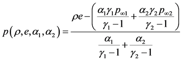 (3.4)
(3.4)
The mixture sound speed corresponds to the Wood (1930) [21] formula:
 . (3.5)
Stiffened gas EOS parameters are determined by the method given in Le Metayer et al. (2004).
It is straightforward to obtain the entropy equations:
 .
.
As System (3.1) is non-conservative, specific relations for its closure in the presence of shocks are needed. In the weak shocks limit, appropriate shock relations have been determined in Saurel et al. (2007) [22] :
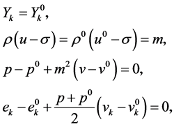 (3.6)
(3.6)
where  denotes the shock speed,
  is the specific volume of fluid k and the superscript ‘0’ denotes the unshocked state.
Even equipped with these relations, this apparently simple model involves many difficulties:
• With the help of relations (3.6), it is possible to solve exactly or approximately the Riemann problem. When dealing with shock propagation in multiphase mixtures, the convergence of the numerical scheme to the exact solution is extremely difficult as the system is non-conservative: The cell average of non-conservative variables has no physical sense. This difficulty appears even with exact Riemann solvers. To reach convergence for shock propagating in multiphase mixtures, a special correction has been developed in Petitpas et al. (2009) [12] .
• Another issue is related to the volume fraction positivity that is difficult to preserve due to the nonconservative term present in the right hand side of the first equation of System (3.1).
In spite of these difficulties, System (3.1) presents very nice features. It is able to create dynamically interfaces as a consequence of the mechanical relaxation process. It involves two entropy equations as well as two temperatures. These properties are important for the extensions to extra physics, as mentioned in the introduction.
To solve System (3.1) for interfaces separating fluids governed by different equations of state, an augmented system is preferred.
3.2. Augmented System
The augmented system with pressure disequilibrium has better properties for numerical resolution than the target system:
• Positivity of the volume fraction is easily preserved.
• The mixture sound speed has a monotonic behavior during the hyperbolic step.
These two properties are key points for the building of a simple, robust and accurate hyperbolic solver. Moreover, with proper treatment of relaxation terms, solutions of the target system (Kapila et al., 2001) [5] will be recovered.
3.3. Flow Model
The augmented model reads:
 (3.7)
(3.7)
The interfacial pressure reads (Saurel et al., 2003 [23] ):
 where
where  represents the acoustic impedance of phase k.
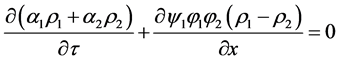
The combination of the two internal energy equations with mass and momentum equations results in the additional mixture energy equation:
 (3.8)
(3.8)
This extra equation will be important during numerical resolution, in order to correct inaccuracies due to the numerical approximation of the two non-conservative internal energy equations.
The phasic entropy equations are readily obtained,
 ,
,  insuring that the mixture entropy
  always evolves with positive or null variations.
This model exhibits a nice feature with respect to the mixture sound speed. The mixture (frozen) sound speed,
 , (3.9)
has a monotonic behavior versus volume and mass fractions.
The model is thus strictly hyperbolic with waves speeds: ,
,  and
and .
.
The numerical resolution of this model is summarized in Section 5, details being available in Saurel et al. (2009). As this model is solved with an Eulerian method, interface capturing results in numerical smearing. In the following section an interface sharpening model is built to remove excessive numerical diffusion.
4. Interface Sharpening
The aim is to build a mathematical model able to sharpen interfaces with the help of Equation (2.6). The subsequent model is not a physical one but a “sharpening model” to reduce artificial diffusion at interfaces. During the sharpening process, mass, momentum and energy will have to be redistributed. To do this, a list of conditions has to be fulfilled:
1) When the initial conditions correspond to a mechanical equilibrium state (uniform velocity and uniform pressure) this state has to remain invariant during the sharpening process. Such initial conditions correspond to those resulting of the hyperbolic flow solver, as interface conditions of equal normal velocities and equal pressures have to be fulfilled.
2) Mass, momentum and energy are redistributed with the help of two contact waves. They must be linearly degenerate in order that the mass, momentum and energy of each phase redistribution be synchronised. The first contact wave will be used for conservative variables redistribution of phase 1 across the artificial shock, the second contact wave will be used similarly for phase 2.
3) The sharpening system must admit a conservative formulation.
4) Mixture mass, momentum and energy must be conserved in a weak sense that will be defined latter.
5) The model must create a single artificial shock, at the interface location.
Before using these various conditions for the model building, a first issue has to be addressed, regarding the link between the sharpening function  and the volume fraction
 .
.
In a sake of clarity we performed the following analysis considering 1-D evolution with . This analysis can be easily extended for the general case detailed in Section 4.6.
4.1. Link between φ and α
The sharpening function  varies between 0 and 1
  and obeys the evolution equation:
 in this particular case of 1D evolutions when
 .
.
The volume fraction  varies between
  and
and :
:  (typically
 ) and obeys the evolution equation:
 .
.
It is important to have non-zero volume fractions for three reasons:
• First, System (3.1) cannot be used at any mesh point if  or
or .
.
• Second, it is useful to have non-zero volume fractions in order to allow dynamic interfaces creation from nearly pure fluids. This is possible with the right hand side of the preceding equation and is important for example in cavitating flow modelling.
• Last, the interface can separate a pure fluid and a mixture of materials, like for example of compacted powder. In this case, the fluid volume fraction in the materials mixture can be far from 0 and 1. An example of interface separating multiphase mixtures will be considered in Section 5.5.
Let us denote by  the difference between the volume fraction on the right and left states far away from the interface:
 . (4.1)
Here  and
and  are limit values of the volume fraction at plus and minus infinity, and in the context of the present assumptions
 .
.
Consider a linear relation between the volume fraction  and the sharpening function
 :
:
 (4.2)
(4.2)
The variation of  is the same as that of
 —it is an increasing function of
 . The equation for
  is similar:
 .
.
Equipped with Relations (4.1) and (4.2) it is now possible to derive the ‘sharpening multiphase model’.
4.2. Sharpening Multiphase Model
Let us consider again the particular case of 1D evolution when . Another important assumption will be done: The volume fraction jump is assumed locally constant,
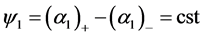 . We will examine later a more general case.
The sharpening multiphase model reads:
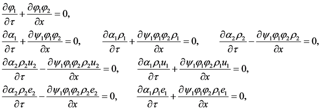 (4.3)
(4.3)
This 8-equation model expresses in non-conservative form as:
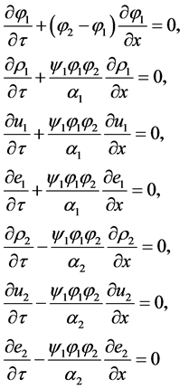 (4.4)
(4.4)
The two internal energy equations can be expressed in terms of pressure equations as, . The calculations are done for the phase 1, similar result being obtained for the second phase:

With the help of the mass equation of phase 1 it becomes:
 .
.
Considering the two pressure equations and the two velocity equations of System (4.4), it appears that for mechanical equilibrium conditions  they reduce to:
 ,
, (4.5)
(4.5)
Therefore, the model clearly respects the most important criterion of the sharpening method, corresponding to the first one of the list given previously: Interface conditions must be unchanged during the sharpening process. In other words, no spurious pressure and velocity oscillations must appear. System (4.3) respects this requirement.
Moreover, the sharpening System (4.4) is hyperbolic with the characteristics:

However, it is not strictly hyperbolic. The fields  are linearly degenerate and the field
  is genuinely non-linear in the sense of Lax. These properties are of paramount importance as will be discussed later.
The waves  correspond to contact waves, responsible for the transport of mass, momentum and energy of each phase.
The flux structure of System (4.3) guarantees synchronised evolutions of the sharpening function, volume fraction, mass, momentum and energy of the various phases.
4.3. Jump Conditions
System (4.3) admits the following set of jump conditions across a discontinuity propagating at speed D:
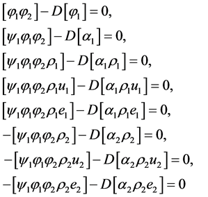 , (4.6)
where, for any function f we denote .
.
4.3.1. Shock Conditions
As shown previously, the first equation of this system admits shocks propagating at the velocity:
 .
.
The second jump condition becomes:
 as
as  has been assumed constant.
Using (4.2), the volume fraction jump is related to the sharpening function jump by,
 .
.
Thus the second jump condition reduces to the first one.
The mass jump condition now becomes:
 .
.
Or,
 .
.
Under expanded form it reads:

It thus reduces to:
 .
.
Across shocks propagating at speed , the jump conditions are thus:
 (4.7)
(4.7)
These jump conditions express that across the sharpening shock, the densities, velocities and internal energies are prolonged. This is a very nice feature already observed with diffuse interface methods. It also means that the pressures are prolonged too. Thus, System (4.7) means that weak solutions of System (4.3) respect interface conditions of equal pressures and equal normal velocities, corresponding to the main criterion the method has to fulfil.
4.3.2. Contact Discontinuities
We now consider contact discontinuities of the sharpening model propagating at speeds . These linearly degenerate waves result in a possible wave pattern as depicted in Figure 4.
For example, for , the first jump condition of System (4.6) becomes:
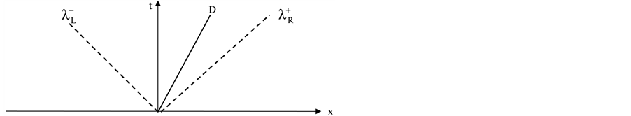
Figure 4. Schematic representation of the Riemann problem wave pattern in the case where .
.
 .
.
As  it becomes,
 .
.
It results in:
 .
.
Consequently,
 (4.8)
(4.8)
System (4.3) thus admits a single shock and two contact discontinuities, corresponding to the one genuinely non-linear field and the two linearly degenerate fields. These various jump conditions will be useful for the Riemann problem (RP) resolution. Before that, let us examine conservation properties.
4.4. Conservation Properties
Summing phase’s mass equations of System (4.3), the mixture mass conservation equation appears:
Denoting the mixture density by  it reads,
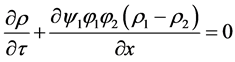 . (4.9)
This equation expresses that the mixture density is going to sharpen during the resolution of System (4.3). However, as the mass transport has already been solved during the diffuse interface model resolution (3.1 or 3.7) no extra mass flux must appear. Equation (4.9) violates the local mass conservation. However, when integrated between the left and right side of the diffuse interface, mass is preserved. Indeed,
 becomes,
 .
.
The same remark holds for phase’s mass, momentum and energy:
 (4.10)
and consequently for the phase’s total energies,
 .
.
The method is thus conservative in the weak sense.
4.6. Summary
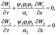
As the sharpening function gradient  is not necessarily positive, the general 1D model reads:
 (4.11)
Jump conditions are the same as previously with obvious modifications related to the  sign.
sign.
5. Riemann Problem and Numerical Scheme
Flows computations proceed in two steps. First the flow model (System 3.7) is solved with Saurel et al. (2009) [6] method as summarized in Section 5.1. During this step, the interface becomes diffused. Thus, during the second step, the sharpening System (4.11) is used to remove most of the numerical diffusion at material interfaces. This system is hyperbolic and conservative. Conventional ingredients of hyperbolic conservation laws can thus be used.
5.1. Numerical Method for the Flow Model
Numerical resolution of the 6-equation augmented model (3.7) in the limit of stiff pressure relaxation has been addressed in Saurel et al. (2009) [6] . This method is particularly robust and quite simple. Computational examples and validations are given in Saurel et al. (2009) [6] and other references cited in introduction, where more sophisticated physical effects are considered.
The system to consider during numerical resolution thus involves 7 equations: System (3.7) and Equation (3.8).
Many approximate Riemann solvers can be considered to determine the cell boundary states, but the HLLC solver of Toro et al. (1994) [24] seems the simplest and the most efficient.
Saurel et al. (2009) [6] method can be summarized as follows:
• At each cell boundary solve the Riemann problem of System (3.7) with HLLC solver.
• Evolve all flow variables with a Godunov type scheme (or its higher order variants).
• Determine the relaxed pressure and especially the volume fraction.
• Compute the mixture pressure with Equation (3.4).
• Reset the internal energies with the computed pressure with the help of their respective EOS.
• Go to the first item for the next time step.
The main drawback of this method is related to the excessive numerical diffusion of interfaces, especially for long time evolutions. The sharpening System (4.11) is addressed in this aim. Its numerical resolution is detailed hereafter.
5.2. Approximate Riemann Solver
Consider a cell boundary separating a left state (L) and a right state (R). At each cell boundary an initial discontinuity is present and three waves are emerging:
• Two contact discontinuities with velocities:
 ,
, 
• A shock wave propagating with speed:
 .
.
For the sake of simplicity we still assume that . Moreover, the function
  that was previously a constant in the entire domain becomes now a local constant:
 . (5.1)
It is important to consider  as a local constant. Indeed, as the volume fraction may vary during the pressure relaxation step, volume fraction jumps may change while the sharpening function will not. This is the reason System (4.11) involves a volume fraction equation and another equation for the sharpening function.
For a given , corresponding to
 , three cases have to be considered:
* , *
, * , *
, *
Let us examine the first situation, the others being similar. The corresponding configuration is depicted in the Figure 4.
The shock speed is determined immediately from the initial data,
 .
.
The sharpening function solution is unchanged compared to the scalar case of Section 2:
 (5.2)
(5.2)
Consequently, the volume fractions are determined as:

System (4.4) can be cast under compact form as:
 (5.3)
(5.3)
with .
.
The approximate Riemann problem solution for variables  thus read:
 ,
, (5.4)
(5.4)
It is worth to mention that in this approximate solution, the solution for  is uncoupled of those of
  and
and .
.
Therefore, when , whatever the situation is (
 or
or  or
or ), the approximate Riemann problem solution is always given by (5.2) and (5.4). The determination of the exact Riemann problem solution is possible, but not necessary for numerical purpose. For the Godunov method, only the flux along the
  axis is needed. Consequently the solution simplifies considerably and is summarised hereafter (below, superscript * represents the solution along the
  trajectory):
Compute If
If ,
,
 ,
,  ,
,  ,
, .
.
If ,
,
 ,
,  ,
,  ,
, (5.5)
(5.5)
Compute If
If ,
,  ,
, .
.
If ,
,  ,
, .
.
The fluxes of System (4.11) are thus easily deduced. They are used in the Godunov (1959) method that reads:
 (5.6)
(5.6)
with,


The fluxes  are computed from the Riemann problem solution (5.4) and contain the appropriate sign function:
 ,
, .
.
The method is stable under conventional CFL restriction based on the fastest wave speed:

Theoretically, the interface is ideally sharpened when the steady state solution of (4.11) is obtained. For practical computations, a CFL number of 0.9 is used and a single time step is done.
5.3. Relaxation Step
In Section 4.5 we have shown that the sharpening method was not creating spurious pressure and velocity oscillations when the sharpening process was starting from initial data corresponding to mechanical equilibrium state. However, when a shock or an expansion wave interacts with an interface, the velocities and pressures are different on both sides of the interface at the discrete level. Thus, the mass redistribution achieved with the sharpening method is associated to momentum and energy redistribution that are going to produce non-equilibrium states on both sides of the interface. In order to restore mechanical equilibrium conditions, which consequence will be to fulfill the interface conditions of equal normal velocities and equal pressures, the following correction is done:
• The center of mass velocity is computed at each mesh point as,
 and both phase velocity are reset to the centre of mass velocity,
 .
.
• A correction is also needed for the internal energies and volume fractions. Indeed, as the mixture becomes out of pressure equilibrium, a pressure relaxation step is done, exactly in the same way as in Saurel et al. (2009) [6] . The volume fractions at pressure equilibrium are determined. Then the mixture pressure is computed with (3.4) and the internal energies are reset using the phase equation of state.
It means that System (4.11) has been complemented by velocity and pressure relaxation terms, in the same way as System (3.7) and that the limit solution when velocities and pressures are relaxed is used to reset the variables. Such correction is obviously conservative with respect to the masses, mixture momentum and mixture total energy. See for example Saurel and Abgrall (1999) [4] for the details in the context of a slightly different two-phase flow model.
6. One-Dimensional Illustrations
We now consider method validation on various test problems of increasing difficulty. A single pseudo time step with CFL = 0.9 is used. With such a choice the convergence is reached at each time step and the interface is computed in one point.
6.1. Advection of an Interface in a Uniform Pressure and Velocity Flow
A volume fraction discontinuity associated to a mixture density discontinuity is moving in a uniform pressure and velocity flow at 100 m/s. Initially the discontinuity is located at  in a 1 m length tube. This discontinuity separates two nearly pure fluids:
• Liquid water on the left defined by , governed by the stiffened gas EOS parameters with parameters
 ,
, 
• Air on the right defined by  and the EOS parameters
  and
and .
.
In the left chamber, the water volume fraction is set to  and in the right chamber its value is
 , with
 . The uniform pressure is set equal to
 .
.
A mesh involving 100 cells is used. The results are shown in the Figure 5 at time  where the conventional method, without interface sharpening (left column) is compared to the version with sharpening correction (right column).
The sharpening algorithm clearly improves the results as the interface is handled in two points instead of 4 - 5 points. The pressure and velocity fields are maintained invariant.
6.2. Single Phase Shock Tube
The aim of this example is to show that the diffuse interface model with the sharpening algorithm is able to improve solutions of the Euler equations. Let’s consider a shock tube filled with air in both chambers. At initial time a pressure discontinuity is present at  in a 1 m length tube. In the left chamber the pressure is set to 2 atm and to 1 atm in the right one. The density is initially uniform
  as well as the velocity that is zero in the entire domain.
In the Figure 6 the results obtained with a higher order extension of the Godunov scheme with MUSCL reconstruction and Superbee limiter are compared to those of the sharpening method with the two-phase model using two times the same ideal gas EOS with . Results are shown at time
  on a mesh
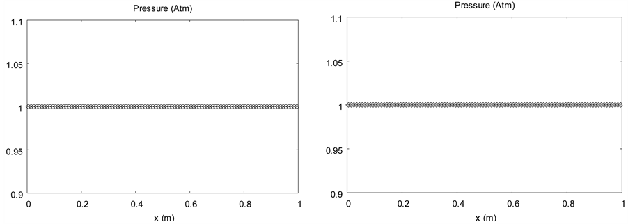
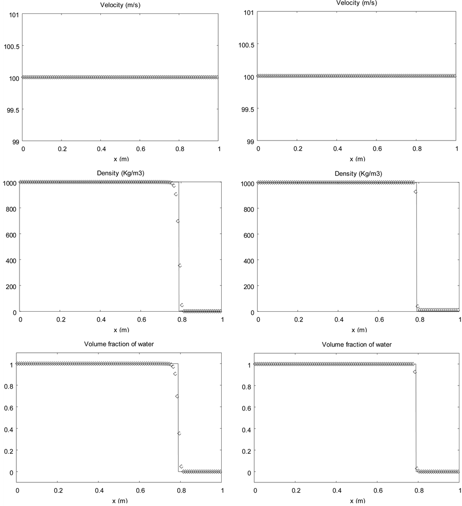
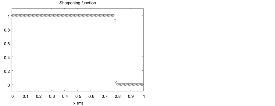
Figure 5. Advection of a volume fraction discontinuity in a uniform pressure and velocity flow. The diffuse interface model without interface sharpening (left column) is solved with the Saurel et al. (2009) [6] method extended to higher order with MUSCL reconstruction and Superbee limiter. The sharpening algorithm is employed for the results of the right column with CFL 0.9 with a single pseudo time step after each step of the diffuse interface solver..
involving 100 cells.
A small oscillation due to the Superbee limiter is present on the velocity graph at shock front when the sharpening algorithm is used. These oscillations are absent with other limiters. Except regarding this discrepancy, the sharpening method improves the results.
6.3. Liquid Water-Air Shock Tube
A 1 m long shock tube containing two chambers separated by an interface at the location  is considered. Each chamber contains a nearly pure fluid. The initial density of water is
  and the stiffened gas EOS parameters are
  and
and . The initial density of air is
  and EOS parameters are
  and
and . The left chamber contains a very small volume fraction of air
  and the initial pressure is set equal to 1 GPa. The right chamber contains the same fluids but the volume fractions are reversed. The initial pressure is set equal to 0.1 MPa. In both chambers the velocity is equal to zero. On Figure 7 the results are shown at time
 . A 1000 cells mesh is used.
A single time step with CFL = 0.9 is done with the sharpening solver after each hyperbolic time step of the diffuse interface model. The interface separating liquid and gas is clearly sharpened, as shown on the mixture density and volume fractions graphs.
6.4. Liquid Water-Air Shock Tube in Extreme Conditions
The same shock tube problem is solved, but initially, the left chamber pressure is set to 1 TPa (10 Mbars). The initial discontinuity is located at .This test illustrates the robustness and convergence of the new algorithm. The results are shown in the Figure 8 at time
  with a mesh using 1000 cells.
Again, the sharpening algorithm clearly improves the solution. An oscillation appears on the mixture density graph with the sharpening method, with similar behavior as Lagrangian and antidiffusion schemes (Kokh and Lagoutière, 2010) [14] . This effect is due to convergence errors that appear during the first time steps, when shock formation occurs. Our method is the only one able to deal with such pressure and density ratio with only one point in the interface.
6.5. Epoxy-Spinel Shock Tube
This test addresses method ability to deal with interfaces separating mixtures of materials. It highlights the need for an evolution equation for the sharpening variable , in addition to the volume fraction variable, both
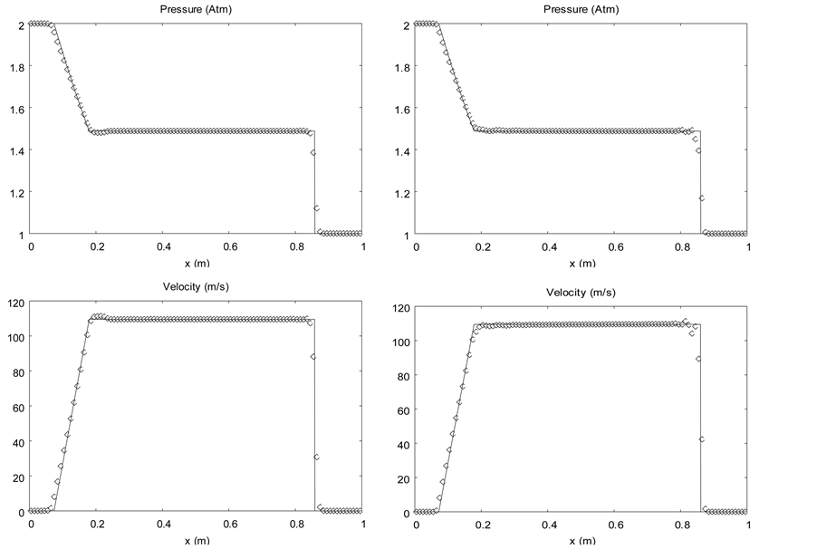
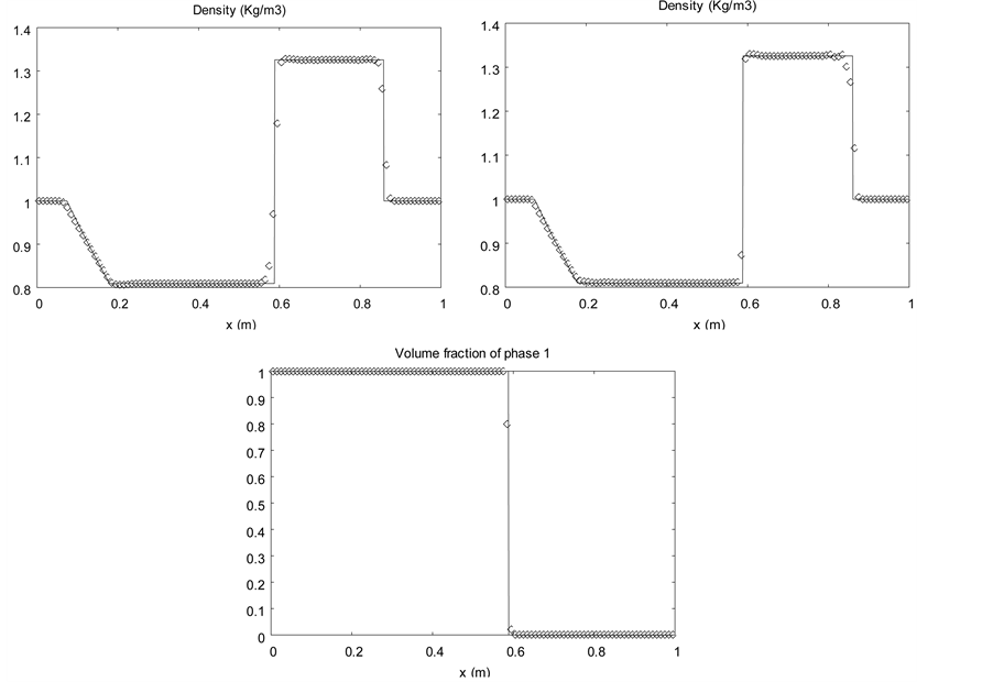
Figure 6. Single phase shock tube. Comparison of a conventional Euler solver (MUSCL reconstruction with Superbee limiter) in symbols (left column) with the sharpening algorithm (with MUSCL reconstruction and Superbee limiter) in the single phase limit (square symbols) shown in the right column for the same variables. The volume fraction is shown for the sharpening algorithm.
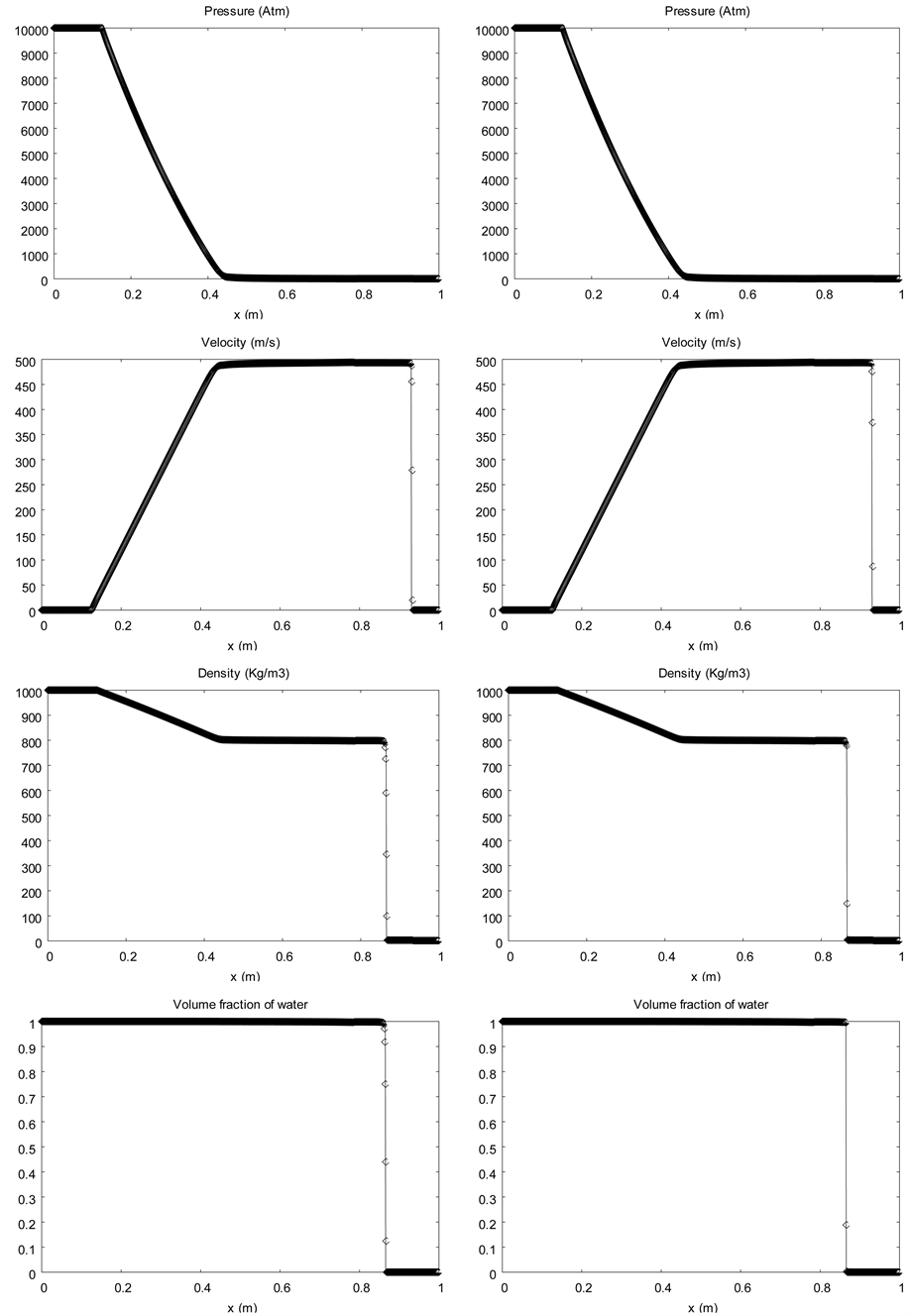
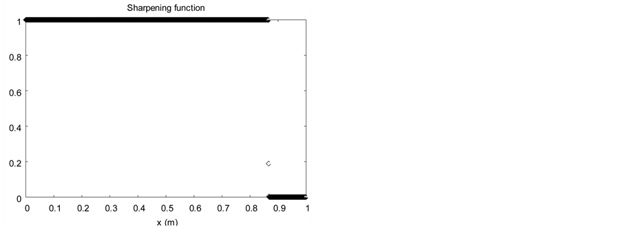
Figure 7. Water-air shock tube. The diffuse interface model without interface sharpening (left column) is solved with the Saurel et al. (2009) [6] method extended to higher order with MUSCL reconstruction with Superbee limiter. The solution with the sharpening algorithm and MUSCL reconstruction with Superbee limiter is shown on the right column.
present in System (4.11).
A 1 m long shock tube containing two chambers separated by an interface at the location  is considered. Each chamber contains a mixture of epoxy and spinel. The initial density of epoxy is
  and the stiffened gas EOS parameters are
  and
and . The initial density of spinel is
  and EOS parameters are
  and
and . The left chamber contains 70% of epoxy in volume and 30% spinel. The initial pressure is set equal to 2 GPa. The right chamber contains the same fluids but the volume fractions are reversed. The initial pressure is set equal to 0.1 MPa. In both chambers the velocity is equal to zero. On Figure 9 the results are shown at time
 . A 400 cells mesh is used.
In this example, the volume fraction and the sharpening function are not anymore linearly dependent. Their dependency is varying with time and space, showing the importance of Relation (5.1). The interface smearing is lowered with the sharp interface method.
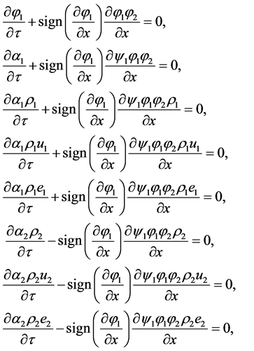
7. More than Two Phases
The multiphase sharpening system can be rewritten as follows:
 ,
,
 ,
,
 ,
,
 ,
,
 .
.
These systems are solved independently for an arbitrary number of fluids. The Godunov method presented in Section 5 results in the fulfilment of the constraints and
and .
.
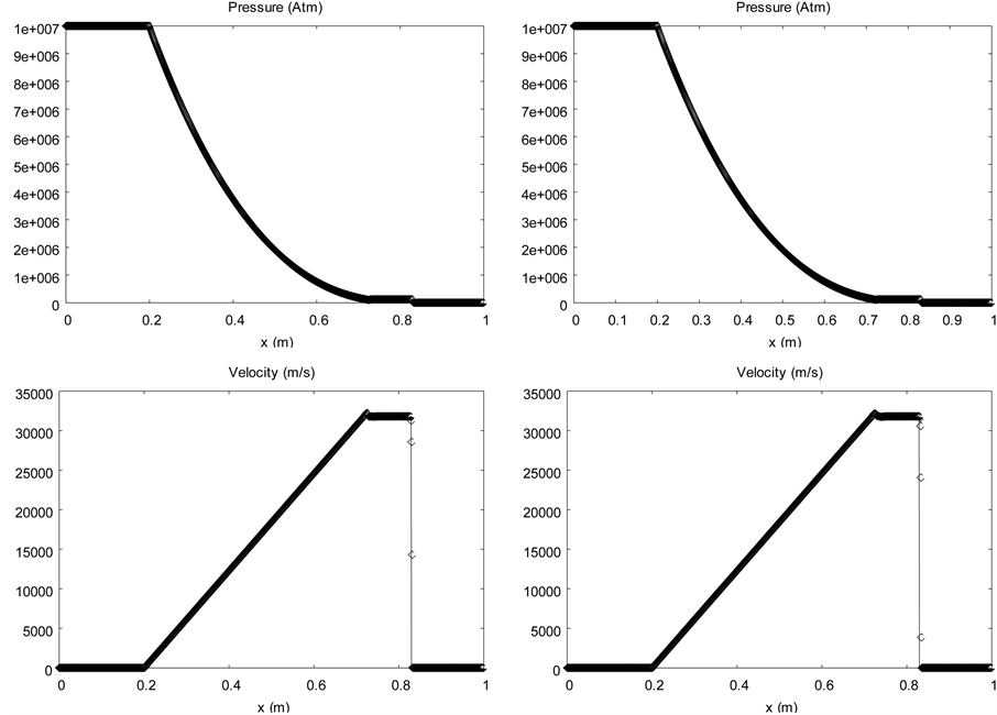
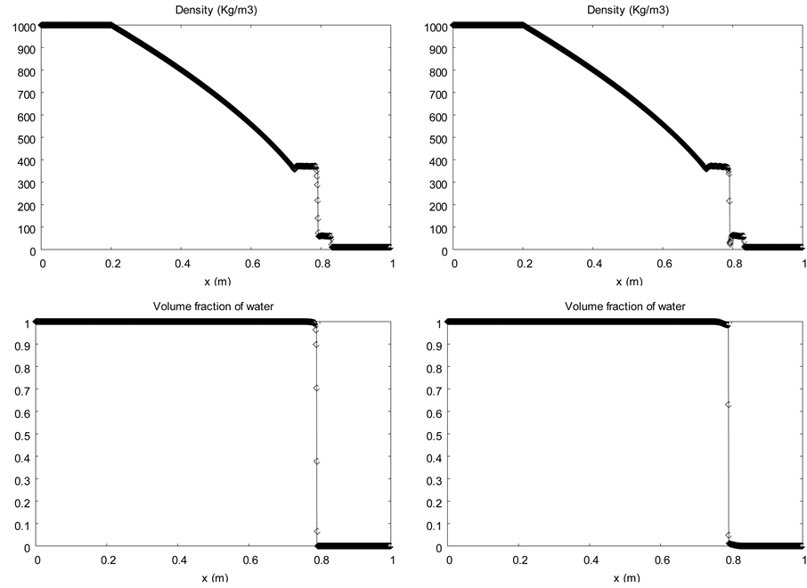
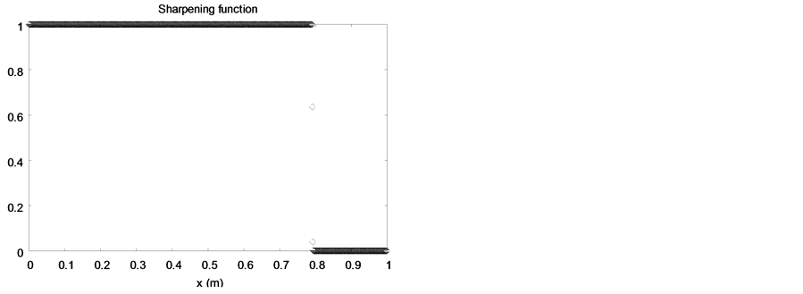
Figure 8. Liquid water-air shock tube in extreme conditions. The diffuse interface model without interface sharpening (left column) is solved with the Saurel et al. (2009) [6] method and extended to higher order with MUSCL reconstruction and Superbee limiter. The solution with the sharpening algorithm and the same MUSCL reconstruction with Superbee limiter is shown on the right column.

Figure 9. Epoxy-spinel shock tube problem. The diffuse interface model (square symbols) without interface sharpening solved with Saurel et al. (2009) [6] method is compared to the solution with the sharpening algorithm (cross symbols) and the exact solution. The same MUSCL reconstruction method with Van Leer limiter is used in both computations.
8. Conclusions
An interface sharpening method has been presented. It is based on Harten (1977 [16] , 1978 [17] ) artificial compression method, and here it is extended to multiphase formulations of diffuse material interfaces (Kapila et al., 2001 [5] , Saurel et al., 2009 [6] ). The key point of the new method is that interface sharpening is achieved in a consistent way with masses, momentum and energies redistribution.
It preserves spurious pressure and velocity oscillations and handles interfaces in about two mesh points. It is also able to handle interfaces separating mixtures of materials.
Multidimensional extension is under examination.
Acknowledgements
This work was partially supported by A * MIDEX and ANR, the grant ANR-11-LABX-0092 and ANR-11- IDEX-0001-02.
References
- Hirt, C.W. and Nichols, B.D. (1981) Volume of Fluid (VOF) METHOD for the Dynamics of Free Boundaries. Journal of Computational Physics, 39, 201-255. http://dx.doi.org/10.1016/0021-9991(81)90145-5
- Youngs, D.L. (1989) Modelling Turbulent Mixing by Rayleigh-Taylor Instability. Physica D: Nonlinear Phenomena, 37, 270-287. http://dx.doi.org/10.1016/0167-2789(89)90135-8
- Fedkiw, R.P., Aslam, T., Merriman, B. and Osher, S. (1999) A Non-Oscillatory Eulerian Approach to Interfaces in Multimaterial Flows (the Ghost Fluid Method). Journal of Computational Physics, 152, 457-492. http://dx.doi.org/10.1006/jcph.1999.6236
- Saurel, R. and Abgrall, R. (1999) A Multiphase Godunov Method for Compressible Multifluid and Multiphase Flows. Journal of Computational Physics, 150, 425-467. http://dx.doi.org/10.1006/jcph.1999.6187
- Kapila, A.K., Menikoff, Bdzil, J.B., Son, S.F. and Stewart, D.S. (2001) Two-Phase Modeling of Deflagration to Detonation Transition in Granular Materials: Reduced Equations. Physics of Fluids, 13, 3002-3024. http://dx.doi.org/10.1063/1.1398042
- Saurel, R., Petitpas, F. and Berry, R.A. (2009) Simple and Efficient Relaxation for Interfaces Separating Compressible Fluids, Cavitating Flows and Shocks in Multiphase Mixtures. Journal of Computational Physics, 228, 1678-1712. http://dx.doi.org/10.1016/j.jcp.2008.11.002
- Perigaud, G. and Saurel, R. (2005) A Compressible Flow Model with Capillary Effects. Journal of Computational Physics, 209, 139-178. http://dx.doi.org/10.1016/j.jcp.2005.03.018
- Braconnier, B. and Nkonga, B. (2009) An All-Speed Relaxation Scheme for Interface Flows with Surface Tension. Journal of Computational Physics, 228, 5722-5739. http://dx.doi.org/10.1016/j.jcp.2009.04.046
- Saurel, R., Petitpas, F. and Abgrall, R. (2008) Modeling Phase Transition in Metastable Liquids. Application to Flashing and Cavitating Flows. Journal of Fluid Mechanics, 607, 313-350. http://dx.doi.org/10.1017/S0022112008002061
- Favrie, N., Gavrilyuk, S. and Saurel, R. (2009) Solid-Fluid Diffuse Interface Model in Cases of Extreme Deformations. Journal of Computational Physics, 228, 6037-6077. http://dx.doi.org/10.1016/j.jcp.2009.05.015
- Favrie, N. and Gavrilyuk, S. (2012) Diffuse Interface Model for Compressible Fluid-Compressible Elastic-Plastic Solid Interaction. Journal of Computational Physics, 231, 2695-2723. http://dx.doi.org/10.1016/j.jcp.2011.11.027
- Petitpas, F., Saurel, R., Franquet, E. and Chinnayya, A. (2009) Modelling Detonation Waves in Condensed Materials: Multiphase CJ Conditions and Multidimensional Computations. Shock Waves, 19, 377-401. http://dx.doi.org/10.1007/s00193-009-0217-7
- Saurel, R., Favrie, N., Petitpas, F., Lallemand, M.H. and Gavrilyuk, S. (2010) Modelling Dynamic and Irreversible Powder Compaction. Journal of Fluid Mechanics, 664, 348-396. http://dx.doi.org/10.1017/S0022112010003794
- Kokh, S. and Lagoutière, F. (2010) An Anti-Diffusive Numerical Scheme for the Simulation of Interfaces between Compressible Fluids by Means of a Five-Equation Model. Journal of Computational Physics, 229, 2773-2809. http://dx.doi.org/10.1016/j.jcp.2009.12.003
- So, K.K., Hu, X.Y. and Adams, N.A. (2012) Anti-Diffusion Interface Sharpening Technique for Two-Phase Compressible Flow Simulations. Journal of Computational Physics, 231, 4304-4323. http://dx.doi.org/10.1016/j.jcp.2012.02.013
- Harten, A. (1977) The Artificial Compression Method for Computation of Shocks and Contact Discontinuities. I. Single Conservation Laws. Communications on Pure and Applied Mathematics, 30, 611-638. http://dx.doi.org/10.1002/cpa.3160300506
- Harten, A. (1978) The Artificial Compression Method for Computation of Shocks and Contact Discontinuities: III. Self-Adjusting Hybrid Schemes. Mathematics of Computation, 32, 363-389.
- Shukla, R.K., Pantano, C. and Freund, J.B. (2010) An Interface Capturing Method for the Simulation of Multi-Phase Compressible Flows. Journal of Computational Physics, 229, 7411-7439. http://dx.doi.org/10.1016/j.jcp.2010.06.025
- Allaire, G., Clerc, S. and Kokh, S. (2002) A Five-Equation Model for the Simulation of Interfaces between Compressible Fluids. Journal of Computational Physics, 181, 577-616. http://dx.doi.org/10.1006/jcph.2002.7143
- Massoni, J., Saurel, R., Nkonga, B. and Abgrall, R. (2002) Proposition de Méthodes et Modèles Eulériens pour les Problèmes à Interfaces Entre Fluides Compressibles en Présence de Transfert de Chaleur: Some Models and Eulerian Methods for Interface Problems between Compressible Fluids with Heat Transfer. International Journal of Heat and Mass Transfer, 45, 1287-1307. http://dx.doi.org/10.1016/S0017-9310(01)00238-1
- Wood, A.B. (1930) A Textbook of Sound. G. Bell and Sons LTD, London.
- Saurel, R., Le Metayer, O., Massoni, J. and Gavrilyuk, S. (2007) Shock Jump Relations for Multiphase Mixtures with Stiff Mechanical Relaxation. Shock Waves, 16, 209-232. http://dx.doi.org/10.1007/s00193-006-0065-7
- Saurel, R., Gavrilyuk, S. and Renaud, F. (2003) A Multiphase Model with Internal Degree of Freedom: Application to Shock-Bubble Interaction. Journal of Fluid Mechanics, 495, 283-321. http://dx.doi.org/10.1017/S002211200300630X
- Toro, E.F., Spruce, M. and Speares, W. (1994) Restoration of the Contact Surface in the HLL Riemann Solver. Shock Waves, 4, 25-34. http://dx.doi.org/10.1007/BF01414629