American Journal of Industrial and Business Management
Vol.3 No.2(2013), Article ID:29898,6 pages DOI:10.4236/ajibm.2013.32019
Study about Economic Growth Quality in Transferred Representative Areas of Midwest China
![]()
1School of Management, University of Science and Technology of China, Hefei, China; 2School of Management, Anhui University of Architecture, Hefei, China.
Email: yuyiyy@126.com
Copyright © 2013 Jun He et al. This is an open access article distributed under the Creative Commons Attribution License, which permits unrestricted use, distribution, and reproduction in any medium, provided the original work is properly cited.
Received December 18th, 2012; revised January 18th, 2013; accepted February 18th, 2013
Keywords: Total Factor Productivity; Malmquist Index; Translog Production Function; Tobit Model
ABSTRACT
Malmquist productivity index (output based) and stochastic frontier production model are used to calculate the total factor productivity and decomposition index of 21 cities in transferred representative area and Shanghai. This paper also uses Tobit model to reveal influencing factors of production efficiency, taking Anhui Province as an example. The result shows that, growth of total factor productivity has been mainly brought by technology progress. Reducing of technology efficiency can hinder its growth. Development gap between Midwest China and developed areas owns to technology efficiency gap. The efficiency has a positive correlation with share of state-owned enterprise total in industrial output value, opening degree, human resources level and infrastructure level. At the same time, it negatively correlates with the share of government spending in GDP. The efficiency is uncorrelated with export and the proportion of science and technology spending accounts for fiscal expenditure.
1. Introduction
After entering the 21 century, China has played an important role in the process of the economic globalization and participated in international competition more and more widely. The economy developed rapidly, with average annual growth rate of 10.2% for GDP from 2000 to 2010. While, along with the advancement of reform and opening up, the imbalance of economic development has been increasing and the district development gap widening. At this moment, the government makes policies to balance the development of different areas. Establishing transferred representative area in Midwest China is one of the policies. This strategy cannot only make full use of geographical advantages, resource and labor of Midwest China, but also promote industrial restructuring upgrading and narrow regional development gap. By the end of 2011, there have been 4 transferred representative areas in Anhui, Guangxi, Hunan Province and Chongqing City respectively. All the 4 areas own resource superiority and location advantages, however these advantages have not been made good use of. Is there any relationship between the economic growth and the efficiency and the technology progress in these areas? What’s the gap between these areas and the developed area? What should the government do to support the economic development to take advantage of these areas? All these questions are needed to be discussed.
TFP, which is the abbreviation of Total Factor Productivity, has been paid more and more attention as a measure of the economic growth quality. In China, empirical studies about total factor productivity mainly focus on three aspects: region, industry and enterprise. Research methods include the Solow Model, DEA (Data Envelopment Analysis) and SFA (Stochastic Frontier Analysis). Ye Yumin [1] uses the Solow Model to measure the national and provincial total factor productivity, thinking that the change of the economic structure could improve the TFP and China’s economic growth depends on capital and technology. Guo Qingwang [2] draws a conclusion that the economic growth gap between different provinces has widened, basing on DEA and kernel density estimation. Meanwhile, he considers that this widened trend is mainly due to different rate of technology progress. Zhao Wei [3] finds that the TFP presents a trend of rise overall and the eastern region grows fastest, at the same time, the technical efficiency has strong convergence. Liu Binglian [4] uses DEA to analyse 196 major cities’ total factor productivity, finding that the urban economic growth still depends on growth of investment, with low efficiency. Wang Zhigang [5] does research on regional efficiency difference and total factor productivity via stochastic frontier analysis, considering that the east is more efficient than the middle and the west. The growth rate of TFP mainly relies on the technology progress rate. Fu Xiaoxia [6] discusses the applicability of DEA and SFA in analyzing China’s economic growth with the provincial panel data. She finds that stochastic frontier analysis is more applicable than data envelopment analysis in total factor productivity measure. Zhou Xiaoyan [7] choose translog production function to study the provincial production efficiency and total factor productivity growth rate, and the result shows that growth rate of total factor productivity is mainly dependent on efficiency rate, while the technology progress rate takes the second place. Wang Zhiping [8] does research on regional characteristics of total factor productivity and efficiency, finding that technological progress is the leading cause of the total factor productivity growth, meanwhile, the effective utilization rate of the foreign investment and infrastructure has an important impact on production efficiency.
Different from that mentioned above, this paper mainly discusses different cities’ total factor productivity and the influence factors of efficiency from 2000 to 2010 through the comparison of the two methods. At the same time, choosing transferred representative areas of Midwest China as object has a certain novelty.
The second part of this essay expounds related theories about DEA-Malmquist index and the stochastic frontier production function in details. The third part takes empirical analysis with panal data to measure total factor productivity growth rate of four transferred representative areas in Midwest China, regarding Shanghai as the benchmarking. The transferred representative area in Anhui province is taken as an example to analyze the influence factors of the technical efficiency via Tobit model. At last, discussions and conclusions are presented.
2. Models
2.1. DEA-Malmquist Index
The method we used was named Malmquist index, after Sten Malmquist, who applied the index to measure the change of consumption in different periods firstly in 1953. Later, some scholars developed the theory, introducing the method into the field of production analysis. Then it became the Malmquist productivity index. The index measures efficiency by calculating the ratio of the output distance function. The distance function can be solved by DEA. The output distance function reflects the distance between the actual output and the optimal output, which can be adopted to measure the size of the technical efficiency. We take technology ST as reference, which presents the production possibility ser. The output distance function in period t is defined as followed:
 (1)
(1)
In Equation (1), x means inputs, y means output and the objective function value θ is the reciprocal of efficiency. Fare, Grosskopf, Norris and Zhang (1994) [9] came up with Malmquist productivity index, which is showed in Equation (2):
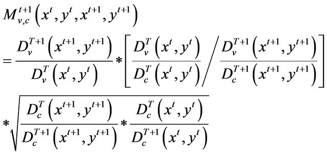 (2)
(2)
In Equation (2), c presents constant return to scale, v presents variable return to scale. The left represents the change of total factor productivity, which can be named as tfpch. The first term in the right represents the change of pure technology efficiency, which can be named as pech, the second term represents the change of scale efficiency, which can be named as sech, the third term represents the change of technology, which can be named as techch. All these indexes indicate that how current value changes when compared with the value in previous period. For instance, if the value of tfpch is greater than 1, the total factor productivity increases. On the contrary, if the value is less than 1, the total factor productivity decreases. Similarly, the other three indexes have the same meaning.
2.2. Decomposition of Total Factor Productivity Based on SFA
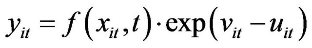
Stochastic Frontier Analysis (SFA) was firstly put forward by Aigner, Lovell and Schmidt [10] and Meeusen, Broeck11 [11] in 1977. Battese and Coelli (1992) [12], Kumbhakar (2000) [13] developed the theory. The model in this paper was summarized by Kumbhakar and Lovell in 2000, which could be displayed in Equation (3):
 (3)
(3)
In Equation (3), yit represents the actual output of firm i in period t.  stands for the deterministic frontier output on the production possibilities frontier. xit means the input of firm i in period t, t means temporal trend. vit represents random error,
  uit represents the inefficiency,
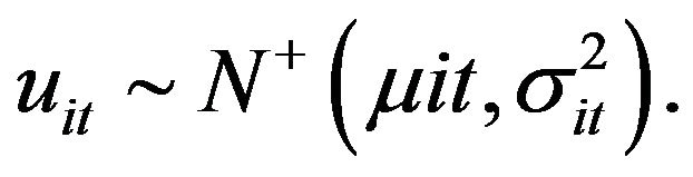
Different from DEA, the form of production function should be set in SFA. Here, we use translog production function to analyze, which is presented as followed:
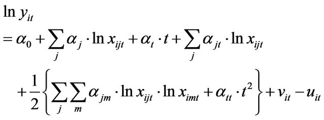 (4)
(4)
In Equation (4), j and m stand for inputs, that is, capital K and labor L in this thesis. According to Kumbhakar (2000), we could decompose total factor productivity growth rate into three parts, that is, the rate of technology progress, the growth rate of technology efficiency and the change rate of scale efficiency. Resource allocation is not taken into account in this paper. The growth rate of total factor productivity can be calculated through following equations:
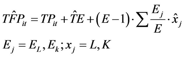 (5)
(5)
 (6)
(6)
In Equation (5), TPit represents technology progress rate, TEit represents the growth rate of technology efficiency, α is parameter. In Equation (6), EL, EK and E represent the output elasticity of labor, the output elasticity of capital and scale elasticity respectively.
3. Empirical Analysis
3.1. Interpretation of Variables and Data
In this paper, we select Shanghai and other 21 cities in Anhui, Guangxi, Hunan and Chongqing as study subjects. Time series starts from 2000 to 2010. All data come from statistic yearbook of each area.
Input variables and output variable. Capital and labor are viewed as input variables, actual gross domestic product (GDP) of each area can be taken as output variable. Here, we choose 2000 as base period. Nominal GDP is converted to Actual GDP using added value index based on the price of 2000. What indicator can stand for the capital stock is a disputed topic. Many scholars utilize perpetual inventory method (PIM) to calculate the value of capital stock. For this method, capital stock of base period, depreciation rate and fixed assets investment price index have a great influence on the result. Meanwhile, in China, most researches select countries or provinces as study objects considering about accessibility of data. Here, we cannot collect relevant data that must be used in PIM, so we substitute the total investment in fixed assets for capital stock. Labor is represented by the number of employees at the end of year.
Variables affect the efficiency. When we take Anhui province as an example to make empirical analysis on the production efficiency, marketization, the degree of openness, government action, human resource level and infrastructure construction are considered as the factors. Share of state-owned industrial enterprise total output value in total industrial output is one of the Market indexes. The proportion of exports in GDP and the share of actual use of foreign investment in GDP could measure the degree of openness. The government behavior can be represented by share of financial expenditure in GDP and the proportion of technology spending in financial expenditure. For the year without the data of technology spending, we substitute the science and technology funds for it. Human resource level could be reflected by average years of schooling of people above 6 years old. Average years of schooling is a weighted average of different levels of education. The weight is the proportion of education degree of people above 6 years old in total population. It multiplies by years of education of different education degree. Years of college degree and above, high school and technical secondary school, junior high school, primary school are 16 years, 12 years, 9 years and 6 years respectively. We utilize principal component analysis to extract indexes that represent infrastructure construction. Original factors contain procession of civil vehicle, postal and telecommunication services, numbers of mobile phone at the end of year and industrial consumption on electricity. All data comes from the statistical yearbooks of Anhui province.
3.2. Consequence of Empirical Analysis Based on DEA-Malmquist Index
The software named Deap2.1 has been used to carry on empirical analysis, which is based on DEA-Malmquist productivity index (input orientated).
Table 1 shows us the technical efficiency growth, technological progress change and total factor productivity growth of Shanghai and four demonstration areas. The data is the average of 11 years from 2000 to 2010. We can find intuitively that the total factor productivity rate of Shanghai increased by 4.0% on average, while other provinces suffered from varying degrees of decline. The total factor productivity of four demonstration areas were down 11.5%, 14.7%, 9.4% and 13% respectively. Development gap between the Midwest and the eastern coastal region is more enormous than the one between the central and western regions. Technical efficiency decline and the technology setback could be taken as decomposition indicators that caused the total factor productivity decline. Concentrating on concrete cities, we can find that the coastal areas and the cities along rivers are better than the inland ones. This may depend on developed trade and ability to attract foreign capital of the coastal areas. Figures 1-3 reflect more specific trends.
Figure 1 shows that the TFP of Shanghai maintains stable growth during 11 years. However, the TFP of other cities rise or fall, presenting a fluctuating trend. Because the market economic system in the eastern coastal cities is more robust than that in the Midwest. We
Table 1. Mean of Malmquist index and decomposition indicators from 2000 to 2010.
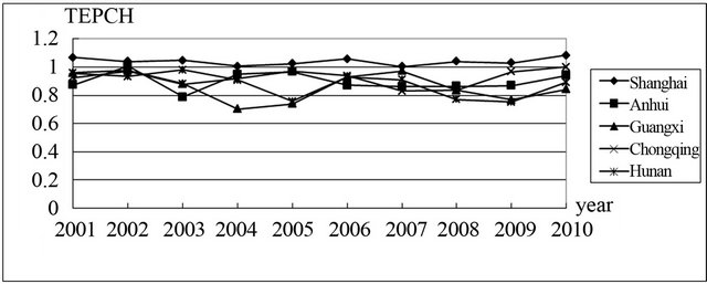
Figure 1. TFP growth rate of each area from 2000 to 2010.
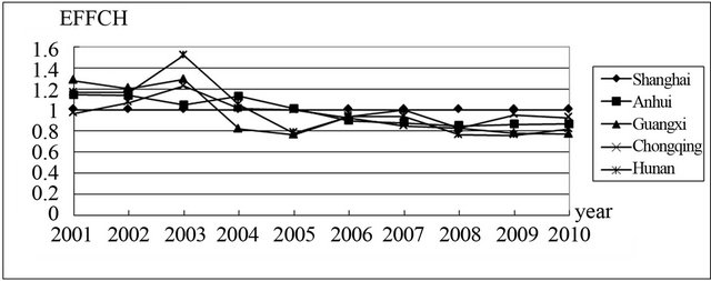
Figure 2. Technology efficiency growth rate of each area from 2000 to 2010.

Figure 3. Technology progress change of each area from 2000 to 2010.
could take notice of three time points, that is 2004, 2007 and 2010. The TFP of most cities declined suddenly in 2004 and 2007. When it came to 2010, the situation took a turn for the better. All these mean that total factor productivity is obviously influenced by the economic cycle, the macro-environment and national policies.
In Figure 2, the growth rate of technical efficiency increased firstly and then decreased, reaching the peak in 2003. Technical change presents an increasing trend in Figure 3. Thus it can be seen that TFP growth mainly relies on technological progress, while it is hindered by the decline in technical efficiency. Technological progress and technical efficiency are reciprocal relationship. Meanwhile, the technology gap between the Midwest and developed regions has greatly narrowed, which is owed to preferential policies. Capital, talent and technology flow to the Midwest. However, technical efficiency of these areas is still low. We should pay more attention to policies that improve the technical efficiency next.
3.3. Results of Stochastic Frontier Analysis
Technical inefficiency items aren’t involved in our study, so we estimate the production function directly, and then measure TFP growth rate, the rate of technological progress, technical efficiency growth and change rate of scale efficiency. Table 2 shows the results of parameter estimation and hypothesis testing.
Table 2. Parameter estimation of translog production function.
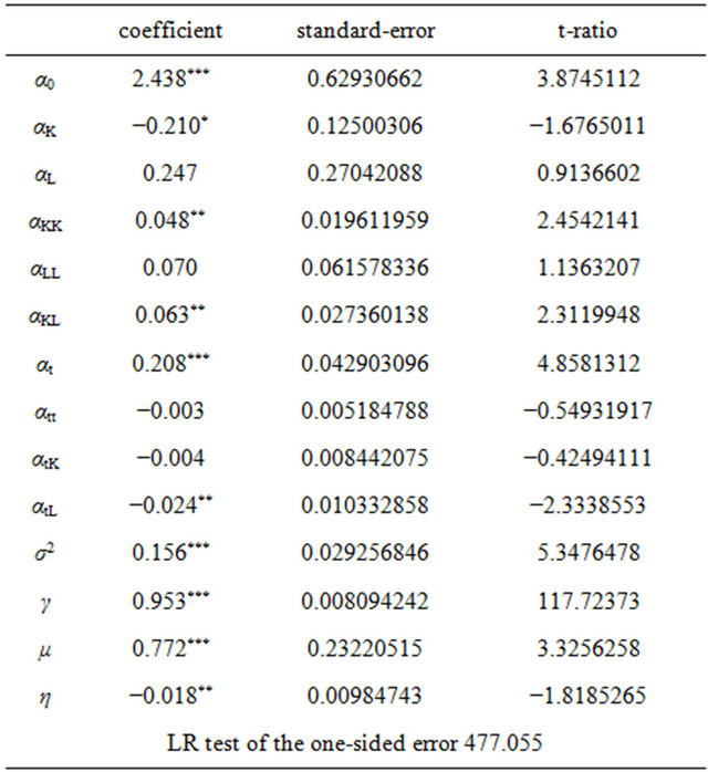
*, **, *** correspond to a significant level of 0.1, 0.05 and 0.01 respectively.
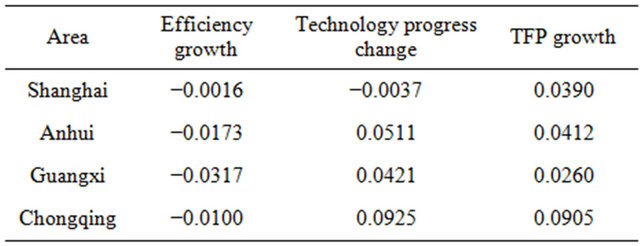
Through the test, the value of γ is 0.953 at the significant level of 0.01, indicating the existence of production inefficiencies. The value of maximum likelihood function is 477.055, indicating the rationality of choosing stochastic frontier production function. According to the coefficient values of the production function arguments in the above, we can calculate the corresponding value of total factor productivity growth and decomposition index, as shown in Table 3.
Comparing Table 3 with Table 1, we find that all the TFP growth during 11 years are plus, which is measured via stochastic frontier production function. The total factor productivity of these cities have improved with little difference. On the other hand, the results of DEA method is different from the one of SFA. The TFP of most regions decline during 11 years except Shanghai. And the gap between Shanghai with other regions is large. In the aspect of a technical efficiency, estimations of technical efficiency through the SFA and DEA both show a downward trend. But the decline through SFA is much smaller than the one through DEA. Technological progress also shows a different trend through different method. DEA derives the outcome of technical regress, while SFA derives an opposite outcome. In addition to Shanghai, other cities showed a certain degree of technical progress, which is more realistic. The reason for this result is that the DEA method does not consider the random factors, which have an significant effect on areas at the cutting edge of technology. Different deterministic frontiers result in different consequences. However, if you want to obtain more detail decomposition indicators of the efficiency, you must use the DEA method.
3.4. Analysis about Factors that Affect Efficiency Based on Tobit Regression
Here, we take transferred cities in Anhui Province as examples for further study on the factors that affect the production efficiency. In general, the efficiency values range between 0 and 1, so we choose Tobit regression as analysis tool. Production efficiency that calculated by the SFA method is treated as explained variable. Exogenous
Table 3. Mean of TFP growth rate and decomposition indicators based on SFA.
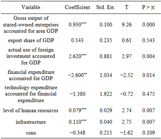
variables reflecting the marketization degree, openness, policies, human resources and infrastructure development are viewed as explanatory variables. Then we establish a regression equation to make an estimation. Analysis result got by the statistical software named Stata 10.0 is presented as followed.
Table 4 shows that production efficiency positively correlates with such variables as the gross output value of state-owned enterprises accounted for the proportion of total industrial output value, share of the actual use of foreign investment accounted for GDP, the level of human resources and infrastructure. Meanwhile, it negatively correlated with the share of financial expenditure accounted for GDP, which may be related to specific items of financial expenditure, such as non-productive expenditure. Neither export share of GDP nor proportion of technology expenditure accounted for financial expenditure has significant correlation with production efficiency. In other words, regions with higher degree of marketization and openness, higher level of human resources and more perfect infrastructure own higher production efficiency. Areas with stronger government intervention have lower production efficiency. It is worth noting that one of our conclusions is different from the ones of existing researches [5,8]. In this paper, there’s a positive correlation between state-owned enterprises proportion of total industrial output value and production efficiency. In our opinion, this may owe to selected areas. Compared with developed regions, state-owned enterprises in the Midwest own more advantages than nonstate-owned enterprises in aspect of industry control, allocation of resources, innovation and R & D.
4. Conclusions
In this paper, the Malmquist index and the stochastic
Table 4. Regression analysis based on Tobit model.
frontier production function have been applied to estimate the total factor productivity growth rate and its decomposition indicators of the industrial transfer demonstration areas and Shanghai. The Tobit model has been used for a further study on factors that affect production efficiency, taking Anhui Province as example. The main conclusions are as follow.
1) Both methods present a upward trend of total factor productivity during the past 11 years. The increase of TFP growth rate mainly relies on technological progress. And the decrease of TFP growth rate owes to technical efficiency decline. At the same time, compared with the developed eastern coastal cities, the technical efficiency of the central and western cities is generally at a low level. Institutional disadvantages may result in the gap, which contains much more government economic intervention, lack of institutional innovation and much more non-productive activities.
2) According to Tobit regression, cities with higher degree of marketization and openness, higher level of human resources and more perfect infrastructure own higher production efficiency. A greater proportion of financial expenditure accounted for GDP generally lowers the production efficiency. Among these variables, the degree of marketization and openness play the most significant role in improving production efficiency. The perfect degree of infrastructure and the level of human resources play a smaller role. Negative effect of government intervention is large.
The conclusions could be viewed as reference when we make policies next. The Midwest regional government should not only pay attention to the increased amount of economic growth, but also focus on the improvement of economic growth quality. They also should not only focus on expansion of the scale, increase of investment in the elements and advancement of technology, but also concentrate on improving the technology efficiency. Meanwhile, we must think highly of the role of institutional innovation for economic growth. Limit government intervention to reduce the negative impact of non-productive activities on production efficiency. Introduce foreign direct investment as well as developed areas inward investment through fiscal and tax preferential policies actively. Guide enterprises to participate in international competition. More government spending should be used for infrastructure construction to provide good public environment for enterprises. Carry on a series of preferential policies to attract talent, which can improve the overall level of regional human resources.
5. Acknowledgements
Our research is sponsored by Natural Science Foundation of Anhui Province. The item number is 11040606M22, which is named “Sustainable development policy research based on the endogenous growth model”. Meanwhile, we thank for the support of Management DepartMent of University of Science and Technology of China.
REFERENCES
- Y. M. Ye, “The Calculation and Analysis of Provincial TFP in China,” Economist, No. 3, 2002, pp. 115-121.
- Q. W. Guo, Z. Y. Zhao and J. X. Jia, “The Analysis of Provincial Total Factor Productivity in China,” The Journal of Word Economy, No. 5, 2005, pp. 46-53.
- W. Zhao, R. Y. Ma and Y. Q. He, “Analysis of Provincial Total Factor Productivity Change: Based on Malmquist Index,” Statistical Research, No. 7, 2005, pp. 37-42.
- B. L. Liu and Q. B. Li, “The Dynamic Analysis of China’s TFP: 1990-2006—Based on Malmquist Index and DEA Model,” Nankai Economic Studies, No. 3, 2009, pp. 139- 152.
- Z. G. Wang, L. T. Gong and Y. Y. Chen, “The Analysis of Provincial Production Efficiency and TFP (1978- 2003),” Social Sciences in China, No. 2, 2006, pp. 55-66.
- X. X. Fu and L. X. Wu, “Adaptability of Frontier Analysis in China’s Economic Growth Accounting,” The Journal of Word Economy, Vol. 7, 2007, pp. 56-66.
- X. Y. Zhou and C. H. Han, “The Decomposition of Production Efficiency and Total Factor Productivity in China (1990-2006),” Nankai Economic Studies, No. 5, 2009, pp. 28-48.
- Z. P. Wang, “Regional Disparity in Production Efficiency and Decomposition of Productivity Growth,” The Journal of Quantitative & Technical Economics, No. 1, 2010, pp. 33-43.
- R. Färe, S. Grosskopf, M. Norris and Z. Zhang, “Productivity Growth, Technical Progress and Efficiency Change in Industrialized Countries,” American Economic Review, No. 84, 1994, pp. 66-83.
- D. Aigner, C. A. Knox Lovell and P. Schmidt, “Formulation and Estimation of Stochastic Frontier Production Function Models,” Journal of Econometrics, Vol. 6, No. 1, 1977, pp. 21-37. doi:10.1016/0304-4076(77)90052-5
- W. Meeusen and J. van den Broeck, “Efficiency Estimation from Cobb-Douglas Production Functions with Composed Error,” International Economic Review, Vol. 18, No. 2, 1977, pp. 435-444. doi:10.2307/2525757
- G. E. Battese and T. J. Coelli, “Frontier Production Functions, Technical Efficiency and Panel Data: With application to Paddy Farmers in India,” Journal of Productivity Analysis, Vol. 3, No. 1-2, 1992, pp. 153-169. doi:10.1007/BF00158774
- S. C. Kumbhakar and C. A. Knox Lovell, “Stochastic Frontier Analysis,” Cambridge University Press, Cambridge, 2003.