Open Journal of Endocrine and Metabolic Diseases
Vol. 3 No. 2 (2013) , Article ID: 31638 , 8 pages DOI:10.4236/ojemd.2013.32018
Etiology and Diagnosis of Major Depression— A Novel Quantitative Approach
Department of Science, Systems and Models, Roskilde University, Roskilde, Denmark
Email: Johnny@ruc.dk
Copyright © 2013 Johnny T. Ottesen. This is an open access article distributed under the Creative Commons Attribution License, which permits unrestricted use, distribution, and reproduction in any medium, provided the original work is properly cited.
Received January 18, 2013; revised February 18, 2013; accepted March 18, 2013
Keywords: Depression; HPA-axis; Etiology; Diagnoses; Clustering analysis; Mixture effect modeling
ABSTRACT
Background: Classical psychiatric opinions are relative uncertain and treatment results are not impressive when dealing with major depression. Depression is related to the endocrine system, but despite much effort a good quantitative measure for characterizing depression has not yet emerged. Methods: Based on ACTH and cortisol levels and using clustering analysis and mixture effect modeling we propose a novel and scientifically based quantitative index, denoted the O-index. The O-index combines a weighted and scaled deviation from normal values in both ACTH and cortisol. Results: Using ANOVA we compare the O-index with opinions reach by classical psychiatric diagnostic procedure (sensitivity 83%, specificity 59%, likelihood ratio positive 2.0, and likelihood ratio negative 0.29). The O-index nicely refines the etiology of depression: Combined with clinical data for 29 subjects earlier reported three categories emerge (p = 4.4 × 10⁻¹³): hypocortisolemic depressed, non-depressed, and hypercotisolemic depressed. The O-index also reveals why it has been difficult to obtain good markers earlier. It explains that healthy subjects may have an elevated (suppressed) level of cortisol or ACTH, however, the healthy system is able to deal with such elevated (suppressed) levels by compensating through suppressing (stimulating) the other component. In contrast the O-index shows that depressed subjects are incapable of making such compensation to a satisfactory degree. We illustrate how the O-index may be used for diagnostic procedure. Discussion: The methods are discussed and based on the available data material we propose that the O-index may be used to improve the diagnostic procedure and consequently the follow-up treatment.
1. Introduction
Depression is a highly complex disease that still requires an exact etiology [1]. It is a widespread disease with serious consequences: recent investigations indicate that 30% - 40% of the population in the Western world experience severe depression at least once in their lifetime [2]. Severe depression significantly affects the social life of the depressed person, sleeping and eating habits, general health as well as family and friends [3]. Depression is a major cause of morbidity worldwide and is very costly for the society [4]. In the United States up to 60% of people who commit suicide have depression or another mood disorder [5]. Due to its relation to other severe diseases, e.g. diabetes and cardiovascular diseases [6-9] and lack of etiology [1] it is associated with a misdiagnosis percentage of at least 30% [10]. Obviously reliable diagnoses are crucial for successful treatment but such reliability has to be based on proper etiology.
Major depression is generally believed to be caused in part by an overactive hypothalamic-pituitary-adrenal (HPA) axis [11,12] but earlier attempts of establishing objective markers for detecting depression based on the hormone levels and pattern produced by the HPA axis have not been successful [12-14]. Investigations indicate that changing levels and patterns of the adrenocorticotrophic hormone (ACTH) and the hormone cortisol secreted by the anterior pituitary and the adrenal glands respectively, are implicated in the pathogenesis of depression [9,14] and that the HPA axis is implicated in cognitive and arousal symptoms [15,16]. Several groups have worked on establishing objective markers related to depression: Ultradian oscillation pattern (characterized by approximately one pulse per 1 - 2 hours) [13], mean concentration of cortisol and ACTH [12,14] and even more advanced methods such as approximated entropy [14] have been suggested. Still no satisfactory quantitative measure for diagnosing depression has yet emerged.
Here we define a novel index denoted the O-index (read “Oh”-index) and show that it may improve the etiology of depression and potentially serve as a reliable and objective marker for diagnosing depression, it may be used to classify individuals into non-depressed subjects, hypercortisolemic depressed subjects and hypocortisolemic depressed subjects. We show that the O-index agrees well with the “classical psychiatric diagnosis method” based on the Carroll Depression Scales (CDS) [17] in combination with mean hormone levels. We also state the probability of false negative and false positive, and show that these are in an acceptable range assuming that the classical method gives correct answers. Two subjects illustrate the potential use in diagnosis and these are compared to classic diagnosis. We conjecture that diagnosis based on the O-index may in fact be less uncertain than classical methods, and that the method will improve not only the reliability of the diagnosis but also the treatment planning and the subsequent effect thereof. The O-index explains that healthy subjects may have an elevated (suppressed) level of cortisol or ACTH, however, the healthy system is able to deal with such elevated (suppressed) levels by compensating through suppressing (stimulating) the other component. In contrast the O-index show that depressed subjects are incapable of making such compensation. Roughly speaking, an elevation (suppression) in the level of either component is not followed by a satisfactory suppression (elevation) in the other component for depressed subjects. Based on the available data material we propose that the O-index may be used for diagnosing depression in the future.
2. Methods
The data encompass 29 subjects (and 2 additional test subjects) and are obtained using the method outlined in [14] where further details may be found: The data are based on two groups, 17 non-depressed and 12 depressed subjects all from North Carolina US. The first group consists of normal healthy adults whereas the second group consists of melancholic and psychotic major depressed adults without any secondary symptoms or diagnosis and who have been free of drug use for sufficient long time. Throughout this paper we simply use the terms “depressed” and “depression” to refer to these subjects when misunderstanding can be avoided. All subjects were studied contemporarily by intensive (10-min) blood sampling for plasma ACTH and serum cortisol measurements over 24 h. All subjects underwent a 24-h blood sampling period starting at 0800 h. Blood was drawn through an indwelling forearm catheter at 10-min intervals for measurement of plasma ACTH and serum cortisol concentrations. Saline infusions at a rate of 50 mL/h were used to keep tubing system patent between all blood samplings. Each sample was immediately centrifuged and stored at −20 C for cortisol and at −80 C for ACTH measurement. Subjects remained at rest, food was given at fixed schedules, mineral water was given ad libitum, and lights were off at 2300 h. Reading and watching television was allowed whereas daytime napping was not allowed. Data from the two additional test subjects used for an illustrative proof of concept was procured.
The data was analyzed using clustering analysis [18,19] and mixture effects modeling [20] combined with standard statistical methods on blinded data as those shown in Figure 1.
The O-index combines a scaled deviation from a normal value in both ACTH and cortisol and we define it as
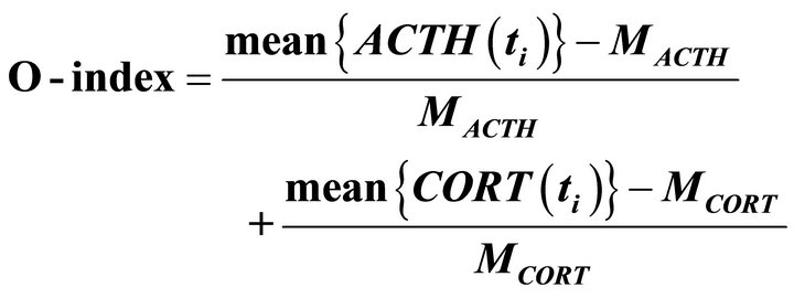
where  and
and  are population average of a 24 h mean of plasma concentration of ACTH and serum cortisol, respectively, over a cohort of non-depressed subjects and
  and
and  are measurement of ACTH and cortisol concentrations at measurements-time
  every 10th minutes for the considered individuals. The means are taken over the available 24 hmeasurements for the individuals considered. Inspired by

Figure 1. ACTH (upper blue curves) and cortisol (lower yellow curves) concentration over 24 hours measured each 10th minute for two randomly chosen subjects. From these data the O-index may be calculated and used for estimating the probability of being hypocortisolemic depressed, hypercortisolemic depressed and for being non-depressed. It turns out that the first subject (the upper pallet) is on the limit between non-depressed and hypocotisolemic depressed and that the second subject (lower pallet) is non-depressed with probability 94%. Data adopted from [11].
the independent investigations [12,14] we take  and
and  as 21 [pg/ml] and 6.1 [μg/dl], respectively.
Cluster analysis evidently divides the n = 29 O-indices into (three) well-defined clusters. Independently a mixture (truncated) density function (11) is derived from data using mixture effect modelling giving the probability that a subject with a given O-index belongs to either of these groups. (Strictly speaking one has to integrate the density function over a tiny interval around the O-index to obtain the probability).
All data used here was assessor blinded, i.e. blinded for the subsequent analysis. After the analysis was finished and conclusions reached the data became unblinded for subsequent comparison reasons. Comparability requires having established a (prior) diagnosis via classical psychiatric methods. By the “classical method” for identifying hypercortisolemic and hypocortisolemic depression we henceforth mean the methods described in [14] (and similar in [11]) where interviews combined with simple mean values of cortisol were used. The results in [14] will serve for comparison studies. Throughout this paper we have used MathWorksMatlab R2012a and built in routines and packages for all calculations done.
3. Results
Independently clustering analysis [18,19] and mixture effect modeling (11) groups O-indices for the assessor blinded data nicely into three well-defined groups; a normo-state (covering normocortisolemia and normocorticotropinemia), a hyper-state (covering hyper-cortisolemia and hypercorticotropinemia), and a hypo-state (covering hypocortisolemia and hypo-cotitropinemia).
3.1. Clustering Analyses
k-means 1D clustering method [18,19] is a metric method which minimizes the sum, over all clusters, of the within-cluster sums of point-to-cluster-centroid distances where by a number of clusters are formed [21] as illustrated in Figure 2 where the horizontal dotted lines divide the one-dimensional data into three clusters hence forth denoted the O-clusters. A dendrogram (not shown) representing the distances between one cluster configuration and its neighbor configurations supported that three O-clusters can be reliably recognized in the present data. Here a configuration refers to an optimal cluster-realization of data for a given number of clusters in the realization. Silhouette values [22] for each point in the clusters, measuring how similar that point is to points in its own cluster compared to points in other clusters confirmed that the three clusters are well constituted.
3.2. Mixture Effect Modeling
In an independent statistical approach using mixture ef-
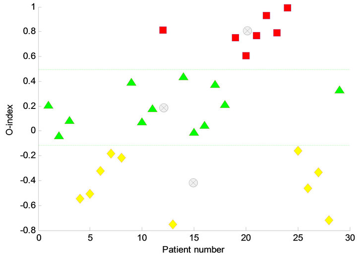
Figure 2. The O-index for 29 subjects and the most likely clustering. The clustering defines three clusters, the O-clusters; a hypo-state corresponding to hypocortisolemic depression (yellow rumps), a normo-state corresponding to non-depression (green triangles) and a hyper-state corresponding to hypercortisolemic depression (pink squares). The three clusters are divided by some threshold values marked by a yellow dotted line. Below the lower yellow dotted line the hypocotisolemic depressed subjects are located and above the upper yellow dotted line the hypercortisolemic depressed subject are located. Between the two dotted lines the non-depressed subjects are located. For each cluster the centroids are shown by light grey encircled crosses.
fect modeling [20] a cumulative empirical distribution function fitting data is obtained and simultaneously the number of model parameters is minimized using Akaike’s Information Criterion (AIC). This approach identifies the same O-clusters as the aforementioned k-means algorithm. Figure 3 shows the best fit consisting of the cumulated distribution function corresponding to the sum of three Gaussians, the 95% confidence curves, and the empirical staircase function. The three corresponding Gaussians and their weights are shown in Figure 4 along with the total density function, i.e. the weighted sum of the individual Gaussians. Means for each of the three Gaussians are μ− = −0.42, μ0 = 0.19 and μ+ = 0.81 respectively, the standard deviations are σ− = 0.21, σ0 = 0.16 and σ+ = 0.12 respectively, and they appear with weights ω− = 0.34, ω0 = 0.41, and ω+ = 0.24 respectively. On the ordinate the O-index of each element in the O-clusters are marked. The n = 29 subjects of the study are divided into three clusters consisting of n− = 10 hypo-state depressed subjects (i.e. belonging to the cluster with lowest O-index), n0 = 12 normo-state subjects (i.e. belonging to the middle cluster representing non-depressed), and n+ = 7 hyper-state depressed subjects (i.e. belonging to the cluster with highest O-index). QQ-plots as well as normal probability plots for each of the O-clusters corresponding to the Gaussians showed satisfactory linear patterns as expected. Thus the O-indices from each of the
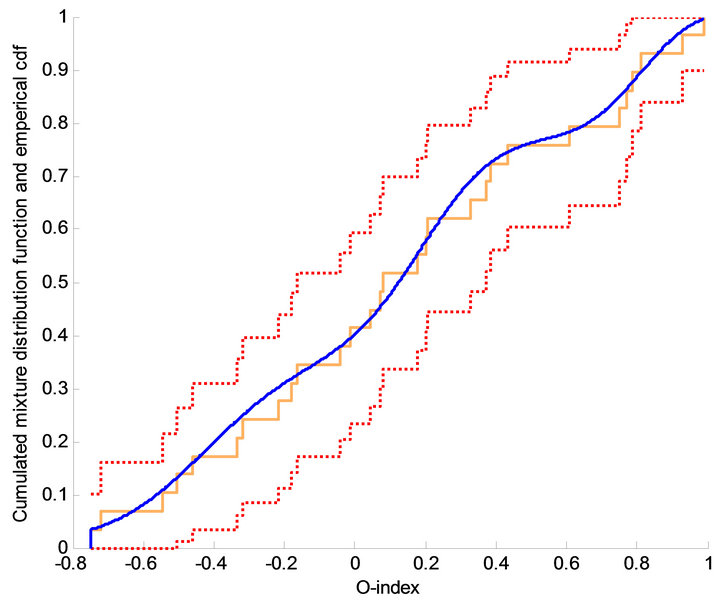
Figure 3. Mixture effect modelling gives the estimated cumulative distribution function fitting data and at the same time minimising the number of model parameters using Akaikes Information Criterion. This approach is independent of the clustering approach but identifies the same clusters as the k-means algorithm. The figure shows the best fit (full blue curve) approximating the cumulative distribution function (orange step curve). The best fit consists of the estimated cumulated distribution function corresponding to the sum of three Gaussians. In addition the 95% confidence curves (dotted curves).
three O-clusters may be considered as normally distributed samples of mutually independent observations.
3.3. Statistical Significance of Three Groups
We may examine if the three groups are statistically different from each other or more specifically whether their means are identical or different by ANOVA (F-tests). To do so, we first have to examine if their variances are equal by Bartlett’s test for homoscedasticity (χ2-tests), since the test for whether their means are equals depends on this result. In conclusion the hypothesis of equal variances cannot be rejected and that the hypothesis of equal means is rejected: The p-value for accepting equal variances between hypo-state, normo-stateand hyper-state (i.e. ) is p = 0.39 (χ2 = 1.90 with 2 degree of freedom). The p-value for accepting equal means between hypo-state, normo-state and hyper-state (i.e. μ− = μ0 = μ+) is p = 4.4 × 10⁻¹³ (F = 103 with (2, 26) degree of freedom). In conclusion, the means of the three O-clusters are significantly different from each other. We may continue by examine whether these distributions are pairwise different from each other by the same strategy as before. The conclusion is that the hypothesis of pairwise equal variances cannot be rejected and that the hypothesis of pairwise equal means are rejected: The p-values for accepting equal variances between hypo-state/normostate (
 ), normo-state/hyper-state (
 ) and hypo-state/hyper-state (
 ) are p = 0.42, p = 0.47 and p = 0.19, respectively. The p-values for accepting equal means between hypo-state/normo-state (μ− = μ0), normo-state/hyper-state (μ0 = μ+) and hypo-state/hyperstate (μ− = μ+) are p = 2.7 × 10⁻⁷, p = 1.2 × 10⁻⁷ and p = 7.2 × 10⁻¹⁰, respectively. Hence the hypothesis of equal means are rejected, meaning that the three O-clusters are pairwise significant different from each other. All the findings are also clearly confirmed by box-plots. We emphasize that both the clustering method and the statistical method give identical groups, the O-clusters, illustrating the robustness and reliability of the O-index.
3.4. Comparison with Classical Method
The classical method using CDS scale [14] divided the subjects into three groups consisting of 17 non-depressed subjects and 12 depressed subjects, where 7 of these depressed subjects was termed hypercortisolemia, i.e. having a mean cortisol concentration above 8 μg/ml, and 5 was termed hypocortisolemia, i.e. having a mean cortisol concentration below 5 μg/ml.
The categories hyper-state depressed and hypo-state depressed based on the O-index identify almost the same cohorts as using the classical method. Assuming that the classical method is correct, we may calculate how well the O-index works, e.g. calculating the probability of false negative and false positive. We find 1) that the O-index shows a high degree of agreement with classical methods on known cohorts of hypercortisolemic and hypocortisolemic depressed subjects (respectively 86% and 80% sensitivity when compared to the other groups); 2) that the few false positive subjects (one in each group) should be characterized as non-depressed due to the Oindex; and 3) that the major deviation appears in the nondepressed cohort (respectively 95% and 75% specificity when compared to the other groups), where respectively 14% and 20% are false negative, which is not alarming compared to the amount of misdiagnosis which generally is at least 30% [10].
The somewhat sparse data set tells us that the O-index is, in itself, not poor in confirming depression (PPV = 59%) compared to CDS; it did correctly identify 83% of all patients diagnosed as depressed by CDS (the sensitivity). The negative result based on the O-index shows that it is good at ensuring that a patient is not diagnosed as depressed (NPV = 83%) in disagreement with CDS but it does only correctly identify 59% of those who are not depressed (the specificity). In addition, the false positive rate (type I error) is 41%, the false negative rate (type II error) is 17%, the likelihood ratio positive is 2.0 (i.e. the sensitivity divided by the false positive rate) and likelyhood ratio negative is 0.29 (i.e. the false negative rate divided by the specificity). These finding are summarized in table 1.
Of cause the method in [14] does not guarantee true diagnosis; in fact, it is putative that psychiatric diagnoses of depression is quite uncertain, partly because of the complexity of mental illnesses and the coupling to other known illnesses [2,6-9] and partly due to lack of etiology. Hence, the deviation between the methods may well be due to uncertainties of the classical methods rather than the proposed O-index. In conclusion we identify the nomo-state with non-depressed subjects, the hypo-state with hypocortisolemic depressed subjects and the hyperstate with hypercortisolemic depressed subjects.
3.5. Diagnostic Illustration
For additional subjects having their O-index measured in the clinic one may use the density function shown in Figure 4 to find the probability that such a subject belongs to the subtypes defined by these O-clusters, i.e. the non-depressed cohort (the normo-state), the hypercortisolemic (the hyper-state) depressed cohort, or the hypocortisolemic (the hypo-state) depressed cohort. As a proof of concept we illustrate this on two additional test subjects adopted from [20] with O-index −0.12 and 0.06, respectively. From the Gaussian density functions identified above the corresponding 95% confidence intervals are [−0.8355, −0.0039] for the hypocortisolemic depressed cohort, [−0.1334, 0.5066] for the non-depressed cohort and [0.5634, 1.0502] for the hypercortisolemic depressed cohort. Thus we estimate that the first test subject may be either hypocortisolemic or non-depressed, none of these possibilities can be statistically rejected using a significance level of α = 5%, but the subject is most unlikely hypercortisolemic depressed. The second test subject is unlikely to be hypocortisolemic or hypercortisolemic depressed but is most likely non-depressed. Since the weighted Gaussians intersects approximately at −0.10 (for hypocortisolemic depressed and non-depressed) and 0.55 (for hypercortisolemic depressed and nondepressed) it turns out that the first test subject has a slightly larger probability (1.4 times bigger) of being hypocortisolemic depressed than being non-depressed. A more specific way to state this is that the posterior probability of the first test subject being hypocortisolemic depressed is approximately 58%, the posterior probability of being non-depressed is 42% and the posterior probability of being hypercortisolemic depressed is 10−10%. Correspondingly for the second test subject the posterior probability of being hypocortisolemic depressed is approximately 6%, the posterior probability of being nondepressed is 94% and the posterior probability of being hypercortisolemic depressed is 10−6%. Here the posterior probability is the value of the weighted density function of interest at the point of observation normalized by the mixture density function at the point of observation. Notice that the first test subject incidentally lies near to the intersection point of the distributions of two cohorts. This is about the worst possible situation with respect to the O-index method. Nevertheless, it is slightly more likely that the first test subject is hypocortisolemic depressed, and it is indeed most likely that the second is non-
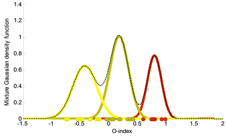
Figure 4. The three corresponding weighted Gaussians are shown along with the total density function, the weighted sum of the individual Gaussians (dotted curve). Means for each of the three Gaussians are −0.42, 0.19 and 0.81 respectively, the standard deviations are 0.21, 0.16 and 0.12 respectively, and they appear with weights 0.34, 0.41, and 0.24 respectively. On the abscissa the O-index of each element in the respective clusters are marked with circles. As a result the subjects are divided into three clusters consisting of 12 non-depressed subjects (green curve), 7 hyper-state depressed subjects (reed curve), and 10 hypo-state depressed subjects (yellow curve).
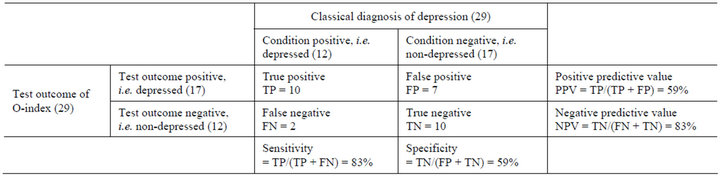
Table 1. Comparison of the two groups of depressed versus non-depressed.
depressed. The outcome of the classical method for these two test subjects was a diagnosis of non-depressed in both cases [11].
Based on the clustering, giving rise to the O-index, one may ask why the more traditional attempts to introduce an index for characterizing depression have failed previously. Keeping the O-clusters fixed we calculate the 2- dimensional Gaussian for each group in the cortisolACTH space given by the 24 h-mean of the normalized deviation in cortisol and ACTH from the average value of a predefined non-depressed cohort respectively (i.e. the first and the second term in the definition of the O-index). The counter plot in Figure 5 reveals three overlapping peaks one for each Gaussian. The centers (located at (−0.18; −0.24), (0.12; 0.07), and (0.25; 0.56) for the hypocortisolemic group, the normocortisolomic group, and the hypercortisolemic group, respectively) of the distributions lies approximately on the diagonal with their minor axis approximately in the same direction and the major axis almost perpendicular to the diagonal ((major axis; minor axis) = ((0.0227, −0.0123); (−0.0123, 0.0151)), ((0.0707, −0.0642); (−0.0642, 0.0820)), and ((0.0515, −0.0172); (−0.0172, 0.0234)) for the hypocortisolemic group, the normocortisolomic group, and the hypercortisolemic group, respectively) as shown in Figure 5. The peaks of the three Gaussians are separated by narrow valleys along the direction of the major axes. Thus trying to define groups directly from either of the
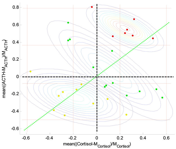
Figure 5. Data and contour plots in the cortisol-ACTH space given by the 24 h-mean of the normalised deviation in cortisol and ACTH from the average value of a predefined non-depressed cohort. The centre of the distributions lies approximately on the diagonal (green dotted line) with their minor axis approximately in the same direction and the major axis nearly perpendicular to the diagonal. By the full reed lines 9 matrix cells are stipulated; low, medium and high cortisol concentrations and low, medium and high ACTH concentrations.
components or from the 2-dimensional pairs consisting of the components would mix up the O-clusters. Hence, if the measurements reflect the depressed state of the subjects then the right point of view is essential that which obtain well-defined groups as is the case with the O-clusters.
3.6. Etiology
Divide the cortisol-ACTH plane into a matrix structure consisting of nine regions, defined by the vertical lines at −0.6, −0.2, 0.2, and 0.6 and horizontal lines at −0.5, 0.07, 0.37, and 0.8 as shown in Figure 5. Thus the hypercortisolemic subjects lies mostly in the high-high region (to the upper right) and a few in the normo-high region (upper-middle). The hypocortisolemic subjects lies roughly either in the low-low region (lower left) or the normolow region (middle-low) but the non-depressed subject lies more spread out roughly in the high-low region (lower-right), the normo-normo region (middle-middle), and the low-high region (upper-left). Hence the majority (i.e. 5 out of 7) of the hypercotisolemic subjects in this study are characterised by having both elevated levels of cortisol and ACTH but there are a minority (i.e. 2 out of 7) having normal level of cortisol but elevated level of ACTH. For the hypocortisolemic subjects the majority have either a suppressed level of both cortisol and ACTH (i.e. 4 out of 10) or a suppressed level of cortisol and a normal level of ACTH (i.e. 4 out of 10). Two hypocortisolemic subjects lie just outside these regions, one having a suppressed level of cortisol and normal level of ACTH (but in the lower end) and the other having a slightly elevated level of cortisol but a suppressed level of ACTH. This observation may give rise to a further subdivision into subcategories and thereby explain intra-variations between the subjects in each O-cluster. However, we will not go further into such speculations here.
As an interesting interpretation of the above observations, we notice that healthy subjects may have elevated level of either cortisol or ACTH but the system are apparently able of dealing with such elevated levels by compensating through suppressing the other component or vice versa. In contrast depressed subjects are not capable of making such compensation. Roughly an elevation in the level of either component is followed by an elevation in the other or similar suppression in either component is follow by suppression in the other one.
4. Discussion
Overall, the results suggest that the O-index may be a reliable, objective and robust marker for defining an etiology for depression with a potential for diagnosing depression as well as the subtypes hypercortisolemia and hypocortisolemia. However, we emphasize that the relative sparse data material entails the possibility of type II error. Furthermore, the data do not meet the standard demands for testing diagnoses but merely those for investigating the aetiology of depression, the selection of the two groups of depressed and non-depressed in the clinical test [14] disregarded subjects with other complications. Clinical experiments as those used here is quite expensive and it has not been possible to find equivalent large scale experiments. But in the near future it is expected that the nanotechnology will make it possible to measure ACTH and cortisol reliable in the perspiration, which are expected to correlate with the corresponding ones in the blood, making such 24 hours studies common during daily settings and thereby promoting large scale investigations.
The mixture density function brings to light the same three clusters as the cluster analysis and it consists of a weighted sum of three Gaussians. The three groups defined by the clusters turns out to be statistically related to non-depressed subjects, hypercortisolemic depressed subjects and hypocortisolemic depressed subjects. The complexity of depression and its coupling to other illnesses should always be taken into consideration when giving a clinical diagnosis. Hence, measuring the O-index should serve only as a supporting factor when deciding on a diagnosis. However, the uniqueness, reliability and robustness of the O-index may make it serve as a very important measurement and therefore the O-index should be taken into consideration if possible when giving a diagnosis. Diagnosis and potential follow-up treatment planning may be improved based on the suggested O-index and likewise pharmaceutical companies could improve their search for new anti-depressive drugs and the effect of these.
5. Acknowledgements
We would like to thank MD Carroll for most kindly letting us use the clinical data reported in [14] and both MD Carrol and MD Veldhuis for encouraging us in performing the present study.
REFERENCES
- N. Sun, Y. Li, Y. Cai, J. Chen, Y. Shen, J. Sun, Z. Zhang, J. Zhang, L. Wang, L. Goo, L. Yang, L. Qiang, Y. Yang, G. Wang, B. Du, J. Xia, H. Rong, Z. Gan, B. Hu, J. Pan, C. Li, S. Sun, W. Han, X. Xiao, L. Dai, G. Jin, Y. Zhang, L. Sun, Y. Chen, H. Zhao, Y. Dang, S. Shi, K. S. Kendler, J. Flint and K. Zhang, “A Comparison of Melancholic and Nonmelancholic Recurrent Major Depression in Han Chinese Women,” Depress Anxiety, Vol. 29, No. 1, 2012, pp. 4-9.
- H. U. Wittchen, F. Jacobi, J. Rehm, A. Gustavsson, M. Svensson, B. Jönsson, J. Olesen, C. Allgulander, J. Alonso, C. Faravelli, L. Fratiglioni, P. Jennum, R. Lieb, A. Maercker, J. van Os, M. Preisig, L. Salvador-Carulla, R. Simon and H.-C. Steinhausen, “The Size and Burden of Mental Disorders and Other Disorders of the Brain in Europe 2010,” European Neuropsychopharmacology, Vol. 21, No. 9, 2011, pp. 655-679. doi:10.1016/j.euroneuro.2011.07.018
- National Institute of Mental Health, US Department of Health & Human Services, National Institutes of Health NIH, “Depression,” 2011. http://www.nimh.nih.gov/health/publications/depression/index.shtml
- World Health Organization, “The World Health Report 2001—Mental Health: New Understanding, New Hope,” Geneva, 2001. http://www.who.int/whr/2001/en/whr01_en.pdf
- D. H. Barlow, “Abnormal Psychology: An Integrative Approach,” 5th Edition, Thomson Wadsworth, Belmont, 2005, pp. 248-249.
- E. Harno and A. White, “Will Treating Diabetes with 11b-HSD1 Inhibitors Affect the HPA Axis?” Trends in Endocrinology and Metabolism, Vol. 21, No. 10, 2010, pp. 619-627.
- J. Jokinen and P. Nordström, “HPA Axis Hyperactivity and Cardiovascular Mortality in Mood Disorder Inpatients,” Journal of Affective Disorders, Vol. 116, No. 1-2, 2009, pp. 88-92.
- R. Rosmond and P. Björntorp, “The Hypothalamic-Pituitary-Adrenal Axis Activity as a Predictor of Cardiovascular Disease, Type 2 Diabetes and Stroke,” Journal of Internal Medicine, Vol. 247, No. 2, 2000, pp. 188-197. doi:10.1046/j.1365-2796.2000.00603.x
- C. M. Pariante and S. L. Lightman, “The HPA Axis in Major Depression: Classical Theories and New Developments,” Trends in Neurosciences, Vol. 31, No. 9, 2008, pp. 464-468. doi:10.1016/j.tins.2008.06.006
- C. L. Bowden, “Strategies to Reduce Misdiagnosis of Bipolar Depression,” Psychiatric Services, Vol. 52, No. 1, 2001, pp. 51-55. doi:10.1176/appi.ps.52.1.51
- D. E. Henley, J. A. Leendertz, G. M. Russell, S. A. Wood, S. Taheri, W. W. Woltersdorf and S. L. Lightman, “Development of an Automated Blood Sampling System for Use in Humans,” al of Medical Engineering & Technology, Vol. 33, No. 3, 2009, pp. 199-208. doi:10.1080/03091900802185970
- M. Deuschle, U. Schweiger, B. Weber, U. Gothardt, A. Körner, J. Schmider, H. Standhardt, C.-H. Lammers and I. Heuser, “Diurnal Activity and Pulsatility of the Hypothalamus-Pituitary-Adrenal System in Male Depressed Patients and Healthy Controls,” Journal of Clinical Endocrinology & Metabolism, Vol. 82, No. 1, 1997, pp. 234-238. doi:10.1210/jc.82.1.234
- R. A. Sarabdjitsingh, F. Spiga, M. S. Oitzl, Y. Kershaw, O. C. Meijer, S. L. Lightman and E. R. De Kloet, “Recovery from Disrupted Ultradian Glucocorticoid Rhythmicity Reveals a Dissociation Between Hormonal and Behavioural Stress Responsiveness,” Journal of Neuroendocrinology, Vol. 22, No. 8, 2010, pp. 862-871.
- B. J. Carroll, F. Cassidy, D. Naftolowitz, N. E. Tatham, W. H. Wilson, A. Iranmanesh, P. Y. Liu and J. D. Veldhuis, “Pathophysiology of Hypercortisolismin Depression,” Acta Psychiatrica Scandinavica, Vol. 115, Suppl. 433, 2007, pp. 90-103. doi:10.1111/j.1600-0447.2007.00967.x
- J. L. Mershon, C. S. Sehlhost, R. W. Rebar and J. H. Liu, “Evidence of a Corticotropin-Releasing Hormone Pulse Generator in Macaque Hypothalamus,” Endocrinology, Vol. 130, No. 5, 1992, pp. 2991-2996. doi:10.1210/en.130.5.2991
- P. Monteleone, “Endocrine Disturbances and Psychiatric Disorders,” Current Opinion in Psychiatry, Vol. 14, No. 6, 2001, pp. 605-610. doi:10.1097/00001504-200111000-00020
- B. J. Carroll, “Carrolls Depression Scales-Revised,” 2004. http://www.psychassessments.com.au/products/21/prod21_report1.pdf
- T. T. Ngo, M. Bellalij and Y. Saad, “The Trace Ration Optimization Problem,” SIAM Review, Vol. 54, No. 3, 2012, pp. 545-569. doi:10.1137/120864799
- D. P. O’Leary, “Scientific Computing with Case Studies,” SIAM Press, Philadelphia, 2009.
- G. J. McLachlan and D. Peel, “Finite Mixture Models,” John Wiley & Sons Inc., New York, 2000. doi:10.1002/0471721182
- R. Matlab, “Statistic Toolbox,” The Math Works, Inc., 2012. http://www.mathworks.se/products/matlab
- L. Kaufman and P. J. Rousseeuw, “Finding Groups in Data: An Introduction to Cluster Analysis,” John Wiley & Sons, Inc., New York, 2005.