Journal of Applied Mathematics and Physics
Vol.2 No.4(2014), Article ID:43723,9 pages DOI:10.4236/jamp.2014.24004
Bessel Function and Damped Simple Harmonic Motion
Masoud Asadi-Zeydabadi
Department of Physics, University of Colorado Denver, Denver, USA
Email: Masoud.Asadi-Zeydabadi@ucdenver.edu
Copyright © 2014 by author and Scientific Research Publishing Inc.
This work is licensed under the Creative Commons Attribution International License (CC BY).
http://creativecommons.org/licenses/by/4.0/


Received 5 February 2014; revised 5 March 2014; accepted 9 March 2014
ABSTRACT
A glance at Bessel functions shows they behave similar to the damped sinusoidal function. In this paper two physical examples (pendulum and spring-mass system with linearly increasing length and mass respectively) have been used as evidence for this observation. It is shown in this paper how Bessel functions can be approximated by the damped sinusoidal function. The numerical method that is introduced works very well in adiabatic condition (slow change) or in small time (independent variable) intervals. The results are also compared with the Lagrange polynomial.
Keywords:Bessel Function; Simple Harmonic Motion; Damped Sinusoidal Function; Lengthening Pendulum; Spring-Mass System; Lagrange Polynomial

1. Introduction
A brief view of the graphs of Bessel and sinusoidal functions shows they are very similar. Bessel functions look like damped sinusoidal functions. Sinusoidal functions are well known for all of us and we have seen the foot prints of them almost everywhere. We knew them from trigonometry but Bessel functions are new for college students and seem more complicated and the students get familiar with them usually in differential equation. Bessel and sinusoidal functions are solution of Bessel and harmonic differential equations. We know these differential equations belong to the family of Sturm-Liouville equation. Bessel and sinusoidal functions are orthogonal function and they appear in the solution of some partial differential equations. The type of orthogonal function that appears in the solution depends on the geometry, physics (the form of the differential equation) and the boundary conditions. In spite of the similarity between them still for the students dealing with Bessel function is more difficult than sinusoidal function.
The purpose of this paper is using a pedagogical method to show the similarity between them through two physical examples. Basically this is an attempt to understand the mathematics through physics. This method is based on the similarity between the form of Bessel and sinusoidal functions and their similarity has been interpreted by these examples. This paper is not aiming to discuss or prove fundamental similarities or differences between these two groups of functions. Basically our observation shows Bessel functions behave like sinusoidal functions with decreasing amplitude and varying period. In this paper two examples are given to understand the root of these behaviors. These examples are the lengthening pendulum and spring-mass system with variable mass. Both length and mass in the pendulum and the spring-mass system respectively increase linearly with time. Finally for these examples the results of the exact solution (Bessel function) are compared with the approximation method (damped sinusoidal function).
In addition to this pedagogical method (physical perspective of Bessel equation) the damped sinusoidal function is a good numerical approximation for Bessel function. It is compared with the Lagrange polynomial fitting; this method provides results better than the Lagrange polynomial fitting.
2. The Lengthening Pendulum
The lengthening pendulum which is known also as Lorentz’s pendulum is similar to a simple pendulum with increasing length  at constant rate
 , with initial length of
  [1] -[8] . Its equation of motion is
 (1)
(1)
where ![]() is the pendulum angle relative to the vertical axis and
is the pendulum angle relative to the vertical axis and ![]() is gravitational acceleration. By changing variable from
is gravitational acceleration. By changing variable from  to
to  and by using the small angle approximation (1) becomes:
 (2)
(2)
The solution of (2) is given by Bessel function as following
 (3)
(3)
where . If
. If  and
and  at
at ![]() then the constants are given by
then the constants are given by  and
and  where
where ![]() is the initial value of
is the initial value of . If
. If  and
and  are related to each other such that
  is a zero of
  then the solution is
 (4)
(4)
where 
To understand the solution in terms of the sinusoidal function, Equation (1) for the small angle approximation can be written as
 (5)
(5)
where  and
and . Notice that since
  is time dependent,
  and
and  are functions of time. If an adiabatic condition (slow change) is considered or if small time intervals are chosen then
  and
and  are almost constant and the equation of motion is similar to damped simple pendulum. Then its solution for under damped condition
  is
is  where frequency of motion is given by
  and it is function of time. For small time interval
  the solution at
  can be written in terms of the conditions of the pendulum at
 :
:
 . This solution shows how Bessel functions can be related to the damped sinusoidal solution.
The equation of motion can also be written in terms of  which is a dimensionless variable as following:
 (6)
(6)
In this case the damping coefficient is . Again under adiabatic condition the solution at the neighborhood of
 ![]() is
is , where
 ,
,  and for
  we have
 . Therefore for large
  the period approaches to
 ![]() like sinusoidal function. By comparing with the exact solution (Bessel function) at the neighborhood of
like sinusoidal function. By comparing with the exact solution (Bessel function) at the neighborhood of ![]() we have:
we have:  where
where
 and
and  are given by the condition of the problem at
![]() . This is an observation based on the solution of the lengthening pendulum and it is not a mathematical proof and depends on two constant (
. This is an observation based on the solution of the lengthening pendulum and it is not a mathematical proof and depends on two constant ( and
and ) that should be determined by the condition at
![]() .
.
3. Spring-Mass System with Linearly Increasing Mass
In this case the mass is increased in steady rate:  where
where  is the initial mass and
 ![]() is the rate of change of the mass. The same treatment as previous case has been used. The equation of motion is:
is the rate of change of the mass. The same treatment as previous case has been used. The equation of motion is:
 (7)
(7)
where  is the spring constant. By changing variable from
  to
to  in (7) we have
 (8)
(8)
The solution of (8) is given by Bessel function as following:
 (9)
(9)
where . The initial conditions of
  and
and  give
give  and
and
 where
where ![]() is the value of
is the value of  at
at![]() . If
. If  and
and  are adjusted such that
is a zero of  then the solution is
 (10)
(10)
where  Equation (7) can be written as
 , (11)
where  and
and . Since
  is time dependent, again
  and
and  are functions of time. The same as the pendulum case for adiabatic condition or for the small time interval
  and
and  are almost constant then the equation of motion is similar to damped harmonic motion. Then its solution for under damped condition
  is
is  where angular frequency of the motion is
  and it is function of time.
The equation of motion in terms of  which is dimensionless is
 (12)
(12)
In this case the damping coefficient is . Again under adiabatic condition the solution at the neighborhood of
 ![]() is
is , where
 ,
,  and for
  we have
 . For large
  the period approaches to
 ![]() like sinusoidal function. By comparing with the exact solution (Bessel function) at the neighborhood of
like sinusoidal function. By comparing with the exact solution (Bessel function) at the neighborhood of ![]() we have
we have  where
where  and
and 
are given by the conditions of the system at![]() . This is physical evidence based on observation and it is not a mathematical proof.
. This is physical evidence based on observation and it is not a mathematical proof.
4. The Quadratic Lagrange Polynomial for Numerical Comparison
In general the damped sinusoidal function provides a good approximation for Bessel functions. It can be compared with the quadratic Lagrange polynomial fitting which is given by [9] [10]
 (13)
(13)
For the quadratic case ![]() and three points,
and three points,  and
and , are needed.
5. Results and Discussion
In this section some results are shown for both cases. The numerical values are used are not based on any physical reason and they are used just for comparison of these two methods.
In both of these problems there are two independent variables ( for pendulum and
  for spring-mass system). Change in the momentum is due to both variables. Appearance of the first derivatives (
 and
and ![]() for pendulum and spring-mass system respectively) make them different from the simple harmonic motion. This is because of the change of the momentum due to the second independent variable (
for pendulum and spring-mass system respectively) make them different from the simple harmonic motion. This is because of the change of the momentum due to the second independent variable ( for the pendulum and
  for the spring-mass system). Mathematically this first derivative plays the role of the damping term that causes the amplitude decay. In reality there is no drag force like air resistance in these two cases but they are not conservative system their energies depend on time [1] . The total mechanical energy is the sum of the kinetic and the potential energy and for the pendulum case the energy density (energy per unit mass) is
 . By substitution of (4) into this expression the energy density is given by
 . The last (Bessel’s) term is proportional to
 ![]() (like kinetic energy). This term decays down and the energy density approaches to
(like kinetic energy). This term decays down and the energy density approaches to . Since
  increases with time the energy decreases. The power density is given by
 . Again the Bessel’s term decays and the power density converges to
  where
where  is the string tension at this limit (at large value of time). Therefore the exact solution shows the energy of the system deceases as we expected from the approximation method based on the damped oscillation. Figure 1 shows the energy density and power density for the case of ν = 0.2048 m/s. It shows power density is negative and it decreases with time and approaches to
  W/kg.
W/kg.
The amplitude decays as  but
but ![]() is inversely proportional to
is inversely proportional to ![]() therefore the rate of the change of the amplitude decreases. The angular frequency
therefore the rate of the change of the amplitude decreases. The angular frequency  increases as
 ![]() increases and approaches to 1,
increases and approaches to 1,  , therefore the period is inversely related to
  (it decreases as
  increases). This means for large
  the amplitude and frequency converge to almost constant values or the solution behaves like simple harmonic motion. We know
  by itself is function of time (
 and
and ) and it increases by time and consequently the period increases by time. This can be clarified by giving the frequencies in terms of (
 and
and ) which are functions of time. The frequencies in terms of
  for the pendulum and the spring-mass system are
  and
and  respectively. For large value of time (large
  and
and ) they approach to
  and
and . That means they get smaller and the periods become larger as time increases.
Figure 2 shows the results of two methods. For these results the small time intervals (less than the local period) have been used. This is a good criterion for the time step size in adaptive numerical method. Figure 2 shows the approximation method (damped sinusoidal method) agrees very well with the exact solution (Bessel function) for small time intervals. One can observe from this figure the period increases with time.
Suppose the pendulum problem has been solved exactly for some initial conditions. This solution is given in (4) by Bessel functions and at a given ![]() the exact conditions of the motion, (
the exact conditions of the motion, (![]() and
and![]() ), can be found and substituted into,
), can be found and substituted into,  , to find
  and
and![]() . Figure 3 shows this solution for
. Figure 3 shows this solution for 
(the first zero of ) with initial conditions of
  and
and . The solution corresponding to
  has been shown by a dot on the graph. At this point the exact and the approximation solutions should
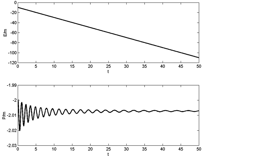
Figure 1. Energy density and power density for the lengthening pendulum: u0 = 30.571 ![]() m/s,
m/s,  and
and
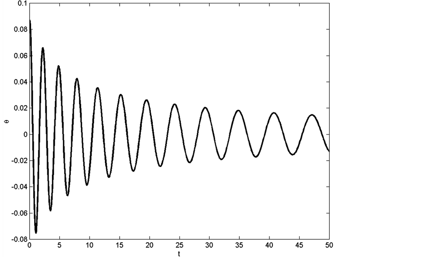
Figure 2. The results of exact (Bessel) and the approximation (damped sinusoidal) solution for the lengthening pendulum (![]()
 m/s,
m/s,  and
and ). Since the small time interval has been used the results of both methods are quite agree with each other (no differences can be seen).
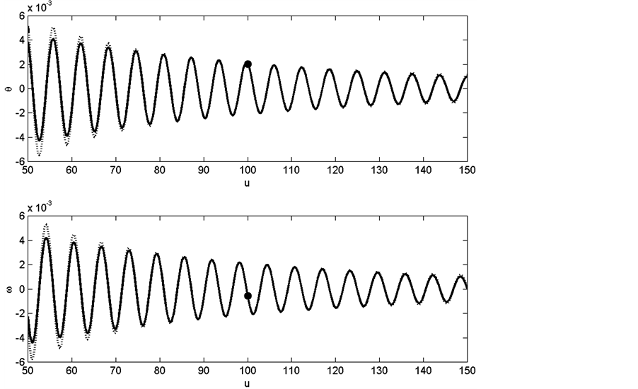
Figure 3. The results of the exact solution, Bessel function (solid line), and the approximation method, damped sinusoidal solution (dot line), for the lengthening pendulum: l0 = 1 m, 

 and
and 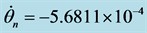 rad/s. The solution corresponding to
  has been shown by a dot on the graph.
match with each other through the condition at ![]() (i.e.
(i.e. ![]() and
and![]() ). Using these conditions from the exact solution and impose them on the approximation (damped sinusoidal) method gives us the approximation solution at the neighborhood of this point. Figure 3 shows the results agree with each other particularly near this point. One can see the deviation of the approximation method from the exact solution away from this point especially for small
). Using these conditions from the exact solution and impose them on the approximation (damped sinusoidal) method gives us the approximation solution at the neighborhood of this point. Figure 3 shows the results agree with each other particularly near this point. One can see the deviation of the approximation method from the exact solution away from this point especially for small . In this case we are not using small time interval and the figure shows the results over several periods.
Figure 4 shows the same results as Figure 3 but for the spring-mass system, in this case the exact solution is given in terms of . Again the results of the exact solution and the approximation method are quite similar. The deviation of these two methods at small
  is shown in Figure 5. Again we can observe for
  the results are matched very well.
In the Lagrange polynomial fitting three points are needed but for the damped sinusoidal function only the value of Bessel function and its derivative at a point are needed. This is a big advantage of this method compare to the Lagrange polynomial fitting. The Bessel function is oscillatory therefore the order of polynomial in a large interval should be higher and more points are needed. Figure 6 shows the comparison of these two techniques with the exact Bessel function.
The results from Figure 6 shows the damped sinusoidal function is a better approximation compare to the Lagrange polynomial fitting. It is obvious for the larger interval the quadratic polynomial is not a reasonable approximation and higher order polynomial with more points are needed. The results of this paper shows in long interval the damped sinusoidal is good numerical approximation.
6. Conclusions
The graphs of Bessel functions are similar to the damped sinusoidal solution. In this paper this observation has been investigated by two physical examples. The Bessel’s equation has been compared with the equation of the damped simple harmonic motion. The solutions of these methods are compared at the neighborhood of an arbitrary point. The results are shown the approximation method works very well particularly when u is large (i.e. for large value of independent variable for example time in this paper for two examples). The damped sinusoidal
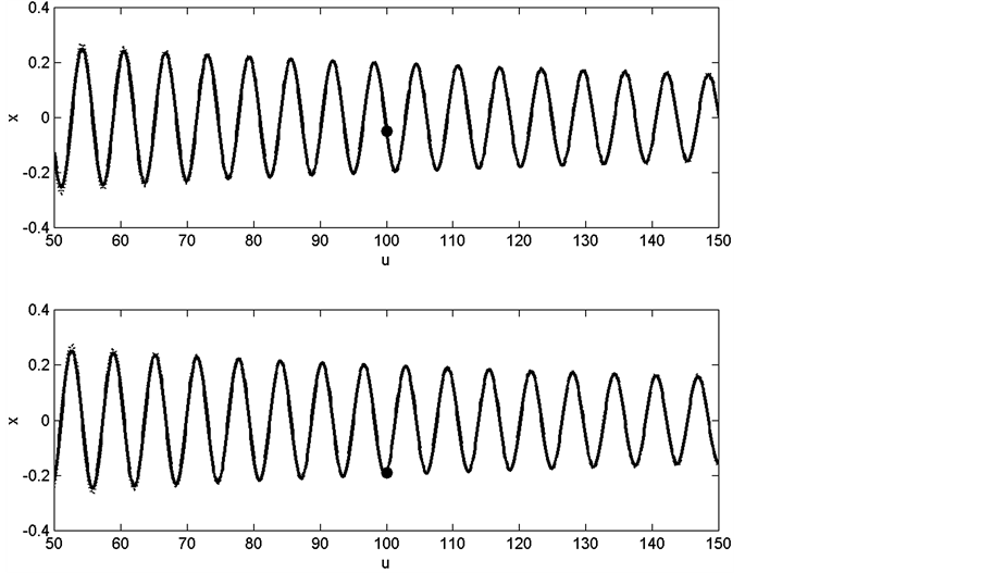
Figure 4. The results of the exact solution (Bessel function, solid line) and the approximation method (damped sinusoidal solution, dot line) for the mass-spring system: m0 = 1 kg, u0 = 3.832, x0 = 1 m, un = 100, xn = −0.0496 m and 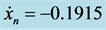 m/s. The solution corresponding to un = 100 has been shown by a dot on the graph.
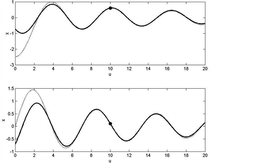
Figure 5. The results of the exact solution (Bessel function, solid line) and the approximation (damped sinusoidal, dot line) method for the mass-spring system: m0 = 1 kg, u0 = 3.832, x0 = 1 m, un = 10, xn = 0.6106 m and  m/s. The solution corresponding to un = 10, has been shown by a dot on the graph.
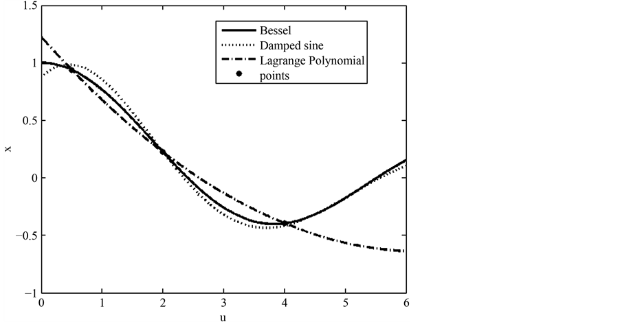
Figure 6. Bessel function, x = J0(u), the damped sinusoidal function, and the quadratic Lagrange polynomial. The given points for Bessel function, J0(0.5) = 0.9385, J0(2.0) = 0.2239 and J0(4.0) = −0.3971, are shown in figure.
function not only is a good way to interpret the property of the Bessel equation but also is a good numerical approximation. The comparison with the Lagrange polynomial shows the numerical advantage of the damped sinusoidal function.
In this paper we use two physical examples but this method can be generalized for any Bessel’s equation. The general form of Bessel’s equation is . Again by using the appropriate initial value for
  the final solution can be given in terms of either
  or
or . The damped sinusoidal solution at the neighborhood of a given point
  is given by (
 ) where
  and
and . The values of Bessel function and its derivative at
 ![]() are used to find
are used to find  and
and![]() . This method can be considered as a good perturbation method for the problems that are involved Bessel function. This method can improve numerical techniques for some particular equations. In the same way we can look at other functions like Legendre polynomial. The Legendre differential equation is given by
. This method can be considered as a good perturbation method for the problems that are involved Bessel function. This method can improve numerical techniques for some particular equations. In the same way we can look at other functions like Legendre polynomial. The Legendre differential equation is given by  with
with ![]() . We can write the differential equation in the form damping harmonic oscillation
. We can write the differential equation in the form damping harmonic oscillation  with
with  and
and  . In this case the solution is growing up and the
  increases by
 . Notice that the polynomial is defined in region of
 ![]() .
.
References
- Werner, A. and Eliezer, J.C. (1969) The Lengthening Pendulum. Journal of Australian Mathematical Society, 9, 331- 336. http://dx.doi.org/10.1017/S1446788700007254
- Littlewood, J.E. (1963) Lorentz’s Pendulum Problem. Annals of Physics, 21, 233-249. http://dx.doi.org/10.1016/0003-4916(63)90107-6
- Littlewood, J.E. (1964) Adiabatic Invariance III. The Equation
 . Annals of Physics, 29, 1-12. http://dx.doi.org/10.1016/0003-4916(64)90188-5
 - Littlewood, J.E. (1964) Adiabatic Invariance IV: Note on a New Method for Lorentz’s Pendulum Problem. Annals of Physics, 29, 13-18. http://dx.doi.org/10.1016/0003-4916(64)90189-7
- Littlewood, J.E. (1964) Adiabatic Invariance V. Multiple Periods. Annals of Physics, 30, 138-153. http://dx.doi.org/10.1016/0003-4916(64)90307-0
- Brearley, M.N. (1966) The Simple Pendulum with Uniformly Changing String Length. Proceedings of the Edinburgh Mathematical Society (Series 2), 15, 61-66.
- Sánchez-Soto, L.L. and Zoido, J. (2013) Variations on the Adiabatic Invariance: The Lorentz Pendulum. American Journal of Physics, 81, 57. http://dx.doi.org/10.1119/1.4763746
- Boas, M.L. (2006) Mathematical Methods in the Physical Science. 3rd Edition, Wiley, 598-599.
- Gil, A., Segura, J. and Temme, N. (2007) Numerical Methods for Special Functions. SIAM. http://dx.doi.org/10.1137/1.9780898717822
- Garcia, A.L. (2000) Method for Physics. 2nd Edition, Prentice-Hall, NJ.