International Journal of Intelligence Science
Vol.2 No.4(2012), Article ID:23690,7 pages DOI:10.4236/ijis.2012.24013
Accurately Measuring Inspection Time with Computers
1School of Pharmacy and Medical Sciences, University of South Australia, Adelaide, Australia
2School of Psychology, University of Adelaide, Adelaide, Australia
Email: nicholas.burns@adelaide.edu.au
Received June 5, 2012; revised August 5, 2012; accepted August 16, 2012
Keywords: Inspection Time; Mental Chronometry; Intelligence; Mental Speed
ABSTRACT
Accurately measuring inspection time (IT) with computers requires several considerations. They are: 1) Screen redraw period; 2) Synchronous and timely image presentation; 3) Stimulus duration timing; 4) Image scale invariance; 5) Stan dardized presentation format (of which image scale invariance is a part). The first consideration dictates a minimum duration available for measuring IT. The second and third are necessary for accurate stimulus duration. The fourth is necessary to provide scale invariant images, that is, images with the same visual angle at a given viewing distance on any computer. And the fifth ensures that participants everywhere respond to the same task. Our computer program embodies these elements and we make it freely available to any interested party. Data to establish validity and reliability are presented, and normative data on 2518 participants aged 6 to 92 years are available.
1. Introduction
Inspection time (IT) is reckoned to index the speed of early stages of information processing. It was conceived and developed by Vickers [1-3] as a component of Vickers’ accumulator model of decision making. IT was considered to estimate the time required for a person to make one observation of sensory input [4], and its implementation has been mainly limited to the visual modality. In the accumulator model, such a quantum of time is said to sum until a critical threshold is reached in favor of a decision. This implies that a decision can be made upon one clean observation of sensory input; albeit with less certainty as the number of discrete samplings is re duced. Over the long term, IT has been shown to correlate about –0.5 with IQ-type measurements [5]. IT is considered an important part of the inventory for measuring individual differences, not the least because it is arguably culturefair (i.e., not influenced by education or socialization). Moreover, the potential of IT as a bio marker for pathological cognitive ageing has been recently raised [6] and investigated [7].
IT measurement has traditionally been implemented by presenting a “pi-shaped” stimulus that has one leg about half the length of the other. The display consists of a brief exposure of an orientating cross (or some such) followed by the stimulus. After some precisely computed interval, the stimulus is masked, and the mask is extinguished upon expiration of a fixed interval (see Figure 1). These are displayed centrally in full-screen mode on a black background (although the use of black stimuli on a white background has been reported [8]). The mask is included to preclude the stimulus iconic afterimage.
The shorter leg of the stimulus is presented with equal probability for either side, and the task is to discriminate on which side the shorter (or longer) leg appeared before being masked. When a participant registers a decision, the sequence reiterates after a one second delay. Response time is irrelevant; participants can reasonably take as long as they like to register a decision. The stimulus is presented for shorter millisecond-periods for correct responses and longer millisecond-periods for incorrect responses, and the algorithm effectively measures the temporal threshold at which a participant can discriminate a difference.
2. Technology
Our program was developed with Microsoft Visual Basic, running under the Windows XP operating system, and exploits the Windows Application Programming Inter face (API) to perform many routines made available through Dynamic Link Libraries (DLLs). These are used by the operating system, and are reused by other applica tions. They provide an efficient solution to many pro gramming tasks. We have also produced an installation package, which ensures that required DLLs, media files and bitmaps are available on a system.
We particularly exploit DirectX, which is an extension of the Microsoft Windows operating system. DirectX is a set of low-level APIs that provide Windows programs with high-performance hardware-accelerated multimedia support. Among the DirectX APIs, Microsoft Direct Draw provides fast access to the accelerated hardware capabilities of a computer’s video adapter.
2.1. Screen Redraw Period
IT can only be measured on a computer in increments of time inversely equal to screen refresh rates. This works because inspection times are characteristically greater than even relatively long screen redraw periods. If the screen is redrawn 100 times per second, say, then the least time a stimulus image can exist before the mask is presented is 10 msec. Hence image duration must be the sum of 10 msec intervals, and image presentation can only occur at the boundary of an interval.
Minimum image duration corresponds to the fastest refresh rate of which a system is capable. Our program enumerates the video card for maximum refresh rate. However, for the program to be effective the monitor needs to be compatible with the computer, that is, it needs to be capable of handling the fast modes of the video card. Notebook computer screens are compatible by design, but a badly matched desktop system may not be compatible.
Our program sets the screen resolution, determined by the video card, for a clear image. When the native screen resolution—best image clarity—does not coincide with maximum refresh rate the program sets the video card to the finest resolution that will operate at maximum refresh rate. Before doing these things, however, it stores the original video card settings and, afterwards, restores them at program termination (see Figure 2). We declare Public dx As New DirectX7, dd As DirectDraw7, ddsd As DDSURFACEDESC2 and then invoke dd. GetDis playMode ddsd, which lists all display modes for the graphics card, from which our program selects the optimal mode.
Figure 3 shows a maximum screen refresh rate of 75 frames per second, with the smallest image duration set to 13 msec (actually, 13.33 msec but rounded forth with). SOA stands for stimulus onset asynchrony; that is, the asynchrony between onsets of two stimuli. Here, it is the duration between stimulus onset and mask onset.
The “Confirmation of settings” box was included so that we could intervene if a computer does not meet the requirements of the IT task. If the user does not click the OK control, the “Confirmation of settings” box persists until the Ctrl-Alt-Esc sequence is pressed. This terminates the program after returning the system to its previous settings. However, this situation is not common, and the program proceeds to the next step at each OK response.
 (a) (b) (c) (d)
Figure 1. Sequence of stimuli presented in the IT task. (a) Orientating cross; (b) Stimulus (left leg shorter form); (c) Mask; (d) Mask blanker.
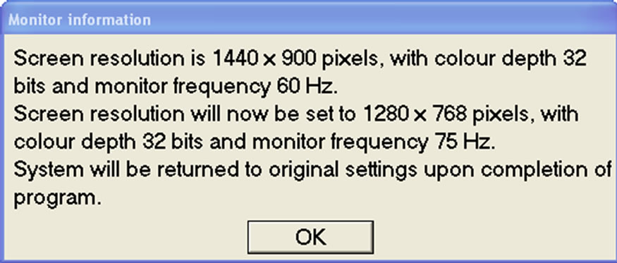
Figure 2. Upon video card enumeration, the message box displays the current screen settings and declares the trial settings.

Figure 3. This message box confirms the trial settings and declares the computed minimum image duration.
2.2. Synchronous and Timely Image Presentation
The second consideration is synchronous and timely presentation. It would be wrong to present the stimulus, or mask, at the instant the screen is halfway through a refresh cycle, for example. The images are centrally located, hence the early part of the last half of the refresh cycle would draw the bottom half of the image and the late part of the first half of the next refresh cycle would draw the top half of the image in that order (and then continue as normal, refreshing the image at the refresh rate). This would interfere with stimulus duration. Even synchronous presentation starting on a given scan line well off the image, for example, does not suffice. Although the image would be drawn all in one go, starting the stimulus timing here would yield the wrong result because of the extra time to scan to the top of the image before presentation. Hence our images are presented when the screen scan line is one line above that which draws the top of the image.
2.3. Stimulus Duration Timing
The third consideration is stimulus duration timing. It would be wrong to start stimulus duration timing at im age presentation, then when the calculated multiple of time intervals terminates, present the mask. The operating system has many demands that result in servicing interrupt requests and allocating time slices to tasks, which would suspend and resume the IT task in a manner normally too quick to detect, but, nevertheless, upset stimulus duration. Before specifically dealing with this, we use timeGetTime in winmm.dll as our program timer. The program sets it to 1 msec update intervals by the call to timeBeginPeriod 1 at the beginning of the actual trial routine. (The timer provided by the program develop ment platform does not allow change of update intervals, and does not have such a fine update interval.) For the time-critical part of the code that displays the stimulus— which we do not want interrupted—we increase our program’s process and thread priorities to maximum by the call to PumpUpTheThreadPriority in perfpres.dll, and, as stated above, start timing when the scan line is one line above that which draws the top of the image. This is de termined by the DirectDraw7.GetScanLine method, which retrieves the scan line that is currently being drawn on the screen. We retrieve these in a program loop until objDraw7Line = rPrimary.Top-1; that is, the scan line number equals the scan line number for the image top minus one. The Windows message loop may delay the frame in which the stimulus is presented, but does little to interfere with timing once the stimulus is presented under maximum process and thread priorities.
The thread priority is restored immediately after mask offset; not after mask onset at stimulus duration timeout because this would compromise a consistent mask duration constituted of the least multiple of minimum image durations sufficient to cover 350 msec. The mask is blanked by a plain black bitmap, which matches the screen background. Thread priority is restored by the call to RestoreThreadPriority in perfpres.dll.
We only elevate the thread priority during this critical bit of code so as to ensure that Windows performs its operating system tasks, but not during execution of the time-sensitive period. After this, and pending participant response, the trial display sequence reiterates. Upon completion of the trial routine, before writing individual and collective participant files, the program restores the update period of timeGetTime to whatever it was origin nally by the call to timeEndPeriod 1.
For TFT/LCD systems, pixels are activated synchronously hence there is no need to check scan lines. However, there is no critical overhead or problem in doing so. Our software satisfies both old and new type displays, and we have found it useful to employ CRT displays in some instances because the fastest are often faster than TFT/LCD systems. Moreover, there is no point in quoting pixel response times for any given TFT/LCD system when they can be different for different systems. As long as they are within the computed screen refresh time for a system, we consider that to be sufficient.
Xie et al. [9] report timing accuracy to within 200 μsec on Windows XP systems. PumpUpTheThreadPriority, in conjunction with timeGetTime and timeBeginPeriod, achieves timing to within 1 msec accuracy on Windows XP platforms running Visual Studio development systems.
2.4. Image Scale Invariance and More Stimulus Duration Timing
The fourth consideration is image scale invariance, which is the size and shape part of a standardized presentation format. If an older computer system can only display 800 × 600 pixels of screen information, and a newer one, 1280 × 1024 pixels, then we do not want images to be displayed in different sizes or aspect ratios between the systems. This is overcome by a device that is also essential for timing accuracy. But first, if we generate images using the draw facility of the program development platform (and generate screen messages by the print facility), then these are dimensioned according to screen resolution; never mind that generating stimulus images upsets timing because of the unknown time taken to generate the images as opposed to outputting them to the screen. Since generation and output are encapsulated in one development platform operation, we could only start stimulus duration timing at the start of image generation. The solution is to write a relatively simple program to generate all active trial images and screen messages, and then screen-copy them to bitmap images using any one of many third-party applications.
Our program preloads these bitmap images onto respective off-screen surfaces of video card memory as an instance of VBDXSurface exposed by DirectDraw. From here, the image required for display is selected as the primary display surface of video memory and is blit (bitblock image transfer) to screen with negligible delay. Video memory is significantly faster than system memory, however we do not copy an off-screen surface to the primary display surface; which would take a little extra time. Our images are displayed by using the hard ware’s ability to flip the visible video surface to an off-screen surface so that the selected image now be comes visible. The off-screen surface becomes the visi ble video surface and the previously displayed video buffer is now the offscreen buffer. This is called page flipping, and is very fast. It is also the other essential feature regarding mask presentation that is necessary for accurate stimulus timing.
Last, we toggle image dimensions between two different presets; one for message display and the other for active trial images. The program does this by selecting corresponding primary display dimensions via our in stance of DDSURFACEDESC2, and the images exhibit the same size and aspect ratios across different screen resolutions and different computer systems. The angular width and height of the stimuli at a viewing distance of one meter are 0.92 deg and 1.26 deg.
Image invariant presentation is accomplished by using the BitBlt method in conjunction with SetPrimDisplay Dimensions SYM_WIDTH, SYM_HEIGHT, which adjusts the image to compensate for different aspect ratios. We do not use standard vector drawing methods because it takes considerably more time to generate and output the images, particularly if compensation for screen aspect ratio was to be included. There are only a few μsecs available between scan line detection and stimulus presentation in which to execute our minimal instruction sequence employed for image presentation. Moreover, our method of image presentation enables us to plug in different stimulus sets for other tasks by simply substituting bitmaps.
While we are aware that subsequent versions of Windows allow programs to be executed under emulations of earlier versions, and that these appear true to the earlier versions, we cannot be sure if timing behavior is replicated. This would need to be tested on new systems. However, we have no problem maintaining suitable Windows XP machines to implement our task and suggest that, at this stage, neither should others. Some fast CRT displays should be included for certain tasks, along with TFT/LCD displays. That a program incorporate the latest technology is unreasonable owing to rapid technological change, hence our considerable investment in a system that provides an enduring platform for tasks where presentation timing is critical. Coming from the birthplace of IT we believe our interpretation to firmly comply with Vickers’ [1,2] intent; especially since he was a colleague of both authors.
3. Implementation
Proceeding in program sequence order, we begin with the dialog box shown in Figure 4, which prompts participants to register entry details. The routine builds filenames from information provided and allows either an ID number-type entry, which can be reckoned against the same ID number for other tests and details, or allows entry of details where the overall test regime has, as yet, no corresponding information. In Figure 4, the latter are initials, birth date and sex. The supervisor has control over which input alternative is disabled (greyed out). The practice box remains ticked for participants, and once their details are complete they click OK to begin a mentored pre-trial routine, which does not let them begin until the supervisor is satisfied that participants under stand what to do. (Input and practice routines can be disabled for maintenance purposes, in which case a standard maintenance filename is created). Supervisors can cancel the program at any time by entering the Ctrl-Alt-Esc sequence, which returns the system to its original configuration. All keyboard input boxes are type-checked for logical violations of character entry, and a participant is prompted to correct an error if one occurs.
Upon clicking OK the program extinguishes the title bar and mouse pointer so as not to cause distraction or interference, and then switches to full-screen, black background mode. (The invisible mouse pointer is constrained to the trial computer screen in case more than one screen is installed.) A mentored pre-trial routine then proceeds. Figure 5 provides an example of instructions presented interactively with the participant’s responses.
Each time a mouse button is pressed, a muted “click” provides operative feedback to the participant. If a participant responds before the mask disappears, they are alerted by a precipitous sound, which is the cue to reenter their response.
3.1. Algorithm for Measuring IT
The algorithm for measuring IT is based upon Wetherill and Levitt [10], and can be understood by reference to a participant’s feedback graph, shown in Figure 6, which
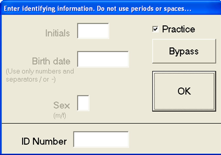
Figure 4. Participant details can be entered in ID number format or Initials, Birth-date, Sex format.
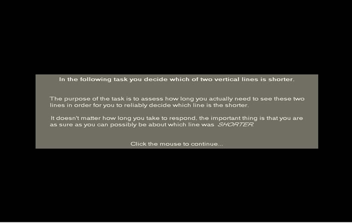
Figure 5. Example of screen format for mentoring instructions used to familiarize participants with task require ments and to meet criterion performance before commencing IT estimation.
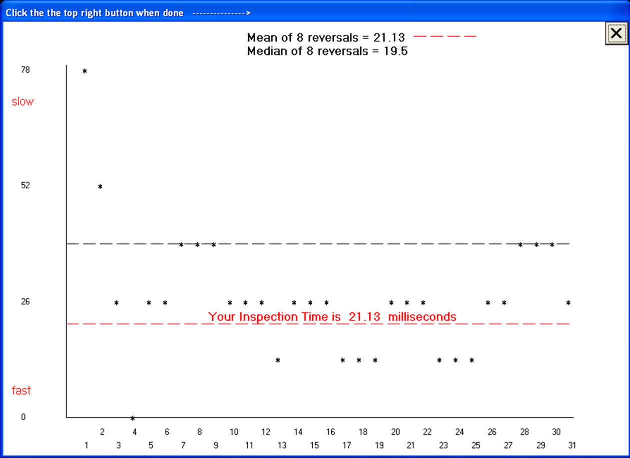
Figure 6. Feedback graph presented to a participant at the end of an IT estimation run. The x-axis indicates trial number and the y-axis indicates msec.
is displayed by the program after measuring IT and saving results. The algorithm starts with a stimulus duration (SD) long enough to be easily discriminated. It is calculated as:

If the smallest SD is 13 msec, then we have 13 × 2 = 26 msec. and the initial stimulus display time is 26 multiplied by the integer part of (100/26) = 26 × 3 = 78 msec. If the smallest SD is relatively long, then it is not multiplied by as much as if it is relatively short. The initial stimulus duration is related to the value 100 msec in such a manner that it is readily discriminated. In this example we continue to work with a smallest SD equal to 13 msec.
As shown in Figure 6, while our participant initially responded correctly the decrement in SD was in intervals of 26 msec. Directly the participant responded incurrectly the first increment of SD was 26 msec, but after wards any change was in 13 msec intervals. The participant needed to get three in a row correct before a decreement. When they got less than three—and as soon as they responded incorrectly—then the interval was incremented and the three-in-a-row rule instituted anew. Of course, when our participant got down to SD = 0 msec (on trial 4) they simply had to guess, and this time their guess was “wrong” thanks to a contrary split from the computer randomizer governing the supposed short leg side.
The program has a special display for SD = 0 msec which makes it appear as if the stimulus and mask are presented simultaneously. Anyway Figure 6 indicates algorithm termination upon eight SD reversals, which was calculated by Wetherill and Levitt [10] to be sufficient for such a task. A participant’s IT is calculated as the mean time in milliseconds of the eight SDs at the reversal points.
Occasionally a participant gets it very wrong with the result that SD increases well above the initial SD, hence the program places an upper limit on SD that cannot be exceeded. If a participant reaches this limit and gets 10 consecutively wrong at the limit, then the estimation run is terminated with a polite message. Maximum SD is calculated as:

Staying with our example, we have 13 multiplied by the integer part of (500/13) = 13 × 38 = 494 msec as the maximum SD. This is also used as the initial SD for the first sequence of practice trials, and is halved for the second sequence of practice trials.
3.2. File Output
Two files types are saved. The first is a common file, which accumulates information for participants. The second is an individual file for each participant, and records their trial history.
For the very first file, that is, if no file exists, the program creates a Dat folder in the same folder as the IT executable and writes the file header in addition to participant information. After this, it simply appends new participant’s information. Autility program can redisplay each participant’s results in the graph format given above upon reading the individual files.
3.3. Windup
The supervisor stays with the participant during the mentoring stage to ensure that they are sufficiently familiar with the task, but departs before the participant clicks the mouse to initiate the trial. Afterwards, the program announces the participant feedback graph with a “windup” refrain loud enough to alert the supervisor that the task is complete, which is the cue to re-enter and briefly explain the results. At this stage the mouse pointer is re-enabled along with the title bar, the latter of which flashes and directs the participant to close the graph when done. After closing the graph a “thank you” screen is displayed, along with a “farewell” riff.
The program embodies many features, such as large message boxes with easy-to-decipher large font and sim- ple messages, but these are not essential to the basics.
4. Validity and Reliability
Our program has been made available to a number of research groups, free-of-charge, on the understanding that we have access to demographic data and IT estimates, and has also been used extensively in our own research program. Most of these studies have yet to be completed hence there are, as yet, no published data us ing our program. However, two examples of validity are the demonstration of differences in IT across individuals; and principled changes of IT with age (specifically, IT improves from childhood to adulthood and then declines with age in later adulthood.
Figure 7 shows a histogram for IT for N = 673 adults (326 females; age range 18 - 45 years, M = 29.2, SD = 9.77 years). Clearly, there is substantial inter-individual variation in IT even in the relatively age-homogeneous young adult sample (for IT, M = 49.0 (SD= 14.5) msec; minimum IT = 14 msec; maximum IT = 156 msec).
Figure 8 shows the distributions for IT in N = 1504 males in ten age groups from under 10 to over 80 years of age. Again, the expected pattern of IT over the lifespan is seen. Together, Figures 7 and 8 demonstrate the validity of IT as measured by our program.
Concerning reliability, the nature of our estimation algorithm, which is an adaptive staircase, precludes estimating internal consistency reliability. However, we have data on test-retest reliability for three samples. First, N = 393, community-dwelling older adults (211 females; age range 65 - 90 years, M = 72.3, SD = 5.55 years) completed two IT estimations separated by six months. The correlation between estimates was r = 0.51. Second, a sample of 30 older adults (17 stroke victims, 13 healthy controls, age range 65 - 90 years, M = 70.7, SD = 9.12
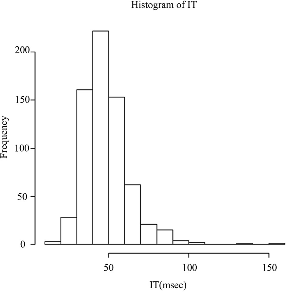
Figure 7. Histogram of inspection time (IT) for N = 673 young adults.

Figure 8. Box-and-whisker plot for N = 1504 males in 10 age groups showing the expected pattern of improvement of IT from childhood into adolescence and adulthood followed by a decline of IT performance in later adulthood.
years) completed two IT estimations separated by six months. The correlation between estimates was r = 0.59. Third, a sample of N = 23 adult males (age range 18 - 38 years, M = 25.3, SD = 6.02 years) completed three estimations within a single experimental session; the average correlation between the three estimates was r = 0.78. As far as we are aware there are no published data on testretest reliability over extended periods for older adults; for younger adults the test-retest reliability we see here is consistent with our own experience using other programs and with estimates in the literature (see, e.g., [5]).
5. Conclusions
In spite of its utility, some researchers [11-13] remark that IT is not the unambiguous measure of time to make one observation of sensory input originally proffered. Upon presentation, the mask interacts with the stimulus to give the illusion that the shorter leg increases length in a flicker of apparent motion, thus suggesting on which side it appeared. Furthermore, the mask interacts with the stimulus to produce a sideways motion away from the longer side towards the shorter side. Hence it may not be minimum discrimination time that is measured, but ability to detect the apparent motion. This can hardly represent time required to inspect something, but rather time required to register a flicker of movement; which is an evolutionary adaptation of many visual systems not all of which can inspect. Whatever the interpretation, such abilities are taken to be related to mental speed, or IQ by way of exploitation of subtle cues, and that is where things stand.
Our program fulfils Jensen’s [14] call for standardizing chronometry insofar as it implements the classical IT task along with the modified mask introduced by Evans and Nettelbeck [15], as well as the Wetherill and Levitt estimation algorithm [10] consistently used at University of Adelaide by Nettelbeck and co-workers. Moreover, it implements sophisticated timing and presentation of the stimuli so that they are invariant and optimal across computers and laboratories.
6. Acknowledgements
The research reported here was supported by Australian Research Council Discovery Grant DP0211113. We are grateful to those who have used our program and have provided some of the data reported herein.
REFERENCES
- D. Vickers, “Evidence for an Accumulator Model of Psychophysical Discrimination,” Ergonomics, Vol. 13, No. 1, 1970, pp. 37-58. doi:10.1080/00140137008931117
- D. Vickers, “Decision Processes in Visual Perception,” Academic Press, London, 1979.
- D. Vickers, T. Nettelbeck and R. J. Willson, “Perceptual Indices of Performance: The Measurement of ‘Inspection Time’ and ‘Noise’ in the Visual System,” Perception, Vol. 1, No. 3, 1970, pp. 263-295. doi:10.1068/p010263
- D. Vickers and P. L. Smith, “The Rationale for the Inspection Time Index,” Personality and Individual Differences, Vol. 7, No. 5, 1986, pp. 609-623. doi:10.1016/0191-8869(86)90030-9
- J. L. Grudnik and J. H. Kranzler, “Meta-Analysis of the Relationship between Intelligence and Inspection Time,” Intelligence, Vol. 29, No. 6, 2001, pp. 523-535. doi:10.1016/S0160-2896(01)00078-2
- T. Gregory, T. Nettelbeck, S. Howard and C. Wilson, “Inspection Time: A Biomarker for Cognitive Decline,” Intelligence, Vol. 36, No. 6, 2008, pp. 664-671. doi:10.1016/j.intell.2008.03.005
- T. Gregory, A. Callaghan, T. Nettelbeck and C. Wilson, “Inspection Time Predicts Individual Differences in Everyday Functioning among Elderly Adults: Testing Discriminant Validity,” Australasian Journal on Ageing, Vol. 28, No. 2, 2009, pp. 87-92. doi:10.1111/j.1741-6612.2009.00366.x
- I. J. Deary and C. Stough, “Intelligence and Inspection Time: Achievements, Prospects and Problems,” American Psychologist, Vol. 51, No. 6, 1996, pp. 599-608. doi:10.1037/0003-066X.51.6.599
- S. Xie, Y. Yang, Z. Yang and J. He, “Millisecond-Accurate Synchronization of Visual Stimulus Displays for Cognitive Research,” Behavior Research Methods, Vol. 37, No. 2, 2005, pp. 373-378. doi:10.3758/BF03192706
- G. B. Wetherill and H. Levitt, “Sequential Estimation of Points on a Psychometric Function,” British Journal of Mathematical and Statistical Psychology, Vol. 18, No. 1, 1965, pp. 1-10. doi:10.1111/j.2044-8317.1965.tb00689.x
- M. White, “Inspection Time Rationale Fails to Demonstrate That Inspection Time Is a Measure of the Speed of Post-Sensory Processing,” Personality and Individual Differences, Vol. 15, No. 2, 1993, pp. 185-198. doi:10.1016/0191-8869(93)90025-X
- M. White, “Interpreting Inspection Time as a Measure of the Speed of Sensory Processing,” Personality and Individual Differences, Vol. 20, No. 3, 1996, pp. 351-363. doi:10.1016/0191-8869(95)00171-9
- N. R. Burns, T. Nettelbeck and M. White, “Testing the Interpretation of Inspection Time as a Measure of Speed of Sensory Processing,” Personality and Individual Differences, Vol. 24, No. 1, 1998, pp. 25-39. doi:10.1016/S0191-8869(97)00142-6
- A. R. Jensen, “Clocking the Mind: Mental Chronometry and Individual Differences,” Elsevier Ltd., Oxford, 2006.
- G. Evans and T. Nettelbeck, “Inspection Time: A Flash Mask to Reduce Apparent Movement Effects,” Personality and Individual Differences, Vol. 15, No. 1, 1993, pp. 91-94. doi:10.1016/0191-8869(93)90045-5