World Journal of Engineering and Technology
Vol.03 No.03(2015), Article ID:58146,9 pages
10.4236/wjet.2015.33012
Study on Fault Location in the T-Connection Transmission Lines Based on Wavelet Transform
Penggao Wen, Hong Song, Zhiting Guo, Quan Pan
School of Automation and Electronic Information, Sichuan University of Science & Engineering, Zigong, China
Email: wpg1018@163.com
Copyright © 2015 by authors and Scientific Research Publishing Inc.
This work is licensed under the Creative Commons Attribution International License (CC BY).
http://creativecommons.org/licenses/by/4.0/


Received 12 May 2015; accepted 15 July 2015; published 21 July 2015
ABSTRACT
The results of T-Line Traveling Wave Fault Location is easily influenced by the wave arrival time and traveling wave propagation velocity; it proposes that the traveling wave uses wavelet transform to extract the modulus maxima of breakdown voltage, to confirm the time of the traveling wave reaching the three-terminal line. The speed of the traveling wave reaching three terminals is confirmed by the structural parameters of the transmission line. We apply the arrival time and propagation velocity to the T-type traveling wave fault location algorithm. Different transmission line distance select the corresponding algorithm, excluding the impact of fault branches and in some cases ranging accuracy, the failure dead zone will not appear. After MATLAB simulation analysis, the algorithm analysis is clear; the range accuracy is high, so that it can meet the requirements of fault location.
Keywords:
Wavelet Transform, T-Connection Line, Traveling Wave Fault, Traveling Wave Fault Location

1. Introduction
In the long-distance transmission system, T-connection transmission lines are a mode of connection which is a higher transport power and heavier load. Once the line fails, there will be a large area power outage, resulting in greater overall social economic losses. Therefore, when the malfunction occurs, we need to identify the fault slip and fault point quickly, and then restore the power, minimize the economic loss and social benefits.
According to the characteristics of T-junction, two aspects of the fault location can be concluded: the judgment of fault slip and the confirmation of failure points. Method One: inject the signal in one end of the circuit; confirm the position of the fault by the start time of the injected signal and the time of signal returns after reaching the point of malfunction. This method has great difficulties of processing data, and the traveling wave in the process of transmission will weaken the signal; the return time of signal is inaccurate [1] . Second method is to use wavelet energy to determine the fault slip, but traveling wave in T line weakens seriously; if the reflected wave calculation error is too large, there are difficulties in the locating [2] . The waveform comparison of wavelet transform modulus maxima is used to remove the impact of the adjacent bus reflected wave. However when the measured line opens circuit in detecting the busbar, the electrical traveling waves can not be detected and the ranging is not confirmed [3] . Because of lack of the above methods, this essay uses the traveling wave caused by the mistake rather than adopts the injection signal directly. We do not need to determine the fault branch directly with the new algorithm, using the voltage traveling wave to avoid the influence of the adjacent bus reflected wave.
The new proposed algorithm has the following advantages: using the voltage traveling wave, eliminating the effects of electrical traveling waves, selecting the appropriate wavelet transform applied to deal with the traveling wave signal [4] , to calculate the time of the traveling wave reaches the three-terminal, and to select the appropriate algorithm by the distance of different transmission line. The calculation is simple, so that there is no dead zone fault and is high accuracy. After doing the simulation research by MATLAB, the results show that this method can confirm the fault branch judgment and fault distance. According to the MATLAB simulation study carried out by this method, the results showed that this method can be determined accurately by judging the distance of the fault and the fault branch.
2. Wavelet Transform
Since the 1990s, the wavelet transform and its engineering applications aroused more and more attention of mathematicians and engineers of various countries, especially in the analysis of power system transient signals, in recent years it has been very good development, and has shown great advantage and potential applications, especially has been a very good development in the electrical equipment fault diagnosis of power quality disturbance signal analysis applications, protection, fault location.
In all of the wavelet transform, continuous wavelet transform, dyadic wavelet transform, orthogonal wavelet transform, semi-orthogonal wavelet transform, different wavelet transform has different characteristics. And in the power transient signal analysis, the wavelet transform is the most important wavelet choice. This paper analyzes the dyadic wavelet transform to select the voltage traveling wave signal.
In the wavelet transform, if  satisfy allowable conditions
 ,
,  is called the wavelet basis or mother wavelet. So the definition of continuous wavelet transform of signal
  is
is
 (1)
(1)
In the formula: , a > 0 is the frequency corresponding to the scale parameter, and b is the time corresponding to the displacement parameters;
  family is a group of wavelet function generated based on wavelet translation and scaling, called wavelet function or wavelet basis.
In the continuous wavelet transform, only the scale parameter do discrete binary ( ,
, ), and the displacement parameters remain continuous change, the resulting semi-discrete wavelet transform form
 (2)
(2)
The wavelet transform is called binary wavelet transform, the corresponding wavelet called binary wavelet, binary wavelet is allowable the wavelet (it satisfies allowable conditions ); Additional binary wavelet should meet the following stability condition: for C, there exist constants A and B, such that:
 (3)
(3)
The function of the stability condition is to ensure the existence of dual wavelet Fourier transform, that is always possible to find a stable dual wavelet reconstructed [5] [6] .
3. Fault Location Algorithm
The Fault Branch’s Judgment
T-connection as shown in Figure 1, A, B, C for the three-terminal system, 1, 2, 3 is measurement points, T is the branch point, the corresponding line length are L1, L2, L3. After a certain point line failure, traveling wave spread to the A, B, C three-terminal, at the measurement point 1, 2, 3 measured traveling wave arrival time of T1, T2, T3. We choose the shortest distance observation point of three observation points as the reference distance point, assuming L1 is the shortest, we choose observation point 1 as a reference observation points. The following discussion is according to the different transmission line distance.
(1) When the three branches are equal, i.e., L1 = L2 = L3. Because traveling wave velocity is equal under the same circumstances, according to T1, T2, T3, we have:
① If T1 = T2 = T3, we can see the point of failure in T node;
② If the time T is equal to the smallest of the three, we can see the fault in time T corresponds to the observation point branch circuit.
(2) When the two branches are equal, assuming TA < TB = TC, we have:
① If the fault happens in slip TA (including node T), it exists time T1 < T2 = T3;
② If the fault happens in slip TB, we choose the observation point 1 as a reference point, we calculate the distance on the line AB and AC fault line distance away from the observation point 1, assuming the distance of the point of fault to the observation point is X, the distance to the node of T is X', according to the same principles of traveling wave velocity [7] , by the following equation holds:
 (4)
(4)
So, we have:
 (5)
(5)
 (6)
(6)
So, we have:
 (7)
(7)
where in , obviously X > L1, due to TB = TC, it is possible that the point of failure is in the TB, is also possible in the TC, then only need to determine the size of T2 and T3 from traveling wave to the observation point of time 2, 3.

Figure 1. T-connection model.
When T2 < T3, the failure points on the line TB; when T2 > T3, the fault on the line TC.
(3) When the two branches are equal, assuming TA > TB = TC, we can know:
① If the fault slip is on TA (including node T) on the existence of time T2 = T3
② If the fault slip is on TB or TC, the algorithm with the (2) ②.
(4) When the three branches are not equal, random selecting L1 < L2 < L3, and we choose the shortest distance observation point of three observation points as the reference distance point. We calculate the distance on the line AB and AC fault line distance away from the observation point 1, assuming the distance of the point of fault to the observation point is X, we have:
① If the fault slip is on TA (including node T), we calculate on the line AB and AC, by Equation (4), we can be obtained:
 (8)
(8)
 (9)
(9)
So X1 = X2, the fault slip is on TA (including node T).
② If the fault slip is on TB, assuming the distance of the point of fault to the node T is X , we calculate on the line AB, by Equation (4) ,we can be obtained:
 (10)
(10)
We calculate on the line AC, by Equation (6), we can be obtained:
 (11)
(11)
So X > L1, the fault slip is on TB.
③ If the fault slip is on TC, assuming the distance of the point of fault to the node T is X , we calculate on the line AC, by Equation (4) ,we can be obtained:
 (12)
(12)
We calculate on the line AB, by Equation (6), we can be obtained:
 (13)
(13)
So X > L1, the fault slip is on TC.
4. The Main Process of Fault Location
The algorithm only need to select the appropriate line, find the corresponding algorithm can quickly find fault branch, and quick and easy calculate, the algorithm simulation process is shown in Figure 2.
5. Matlab Simulate and the Error Analysis
5.1. Simulation Model
To validate the algorithm proposed in this paper, and using MATLAB/Simulink establish 220 KV three-terminal power system model shown in Figure 1. Used binary wavelet transform in simulation, found the corresponding moment after extraction modulus maxiama of phase-mode tansformation about fault voltage. Set the simulation time is 0.03 S, the sampling frequency is 1 MHZ, the start time of fault is 0.01 S. Line parameters: R1 = 0.01273 Ω/km; R0 = 0.3864 Ω/km; L1 = 0.9337 × 10⁻³ H/km; L0 = 4.1264 × 10⁻³ H/km; C1 = 12.74 × 10⁻⁹ F/km; C0 =
7.751 × 10⁻⁹ F/km; velocity of traveling wave is  [8] .
[8] .
1) When the line length is AT = L1 = 120 km, BT = L2 = 100 km, CT = L3 = 100 km, after phase-mode trans- formation and the extraction of maximum modulus by wavelet transform, the simulation diagram of the fault voltage shown in Figure 3.
The calculation results of fault at AT, BT, CT showed in Table 1.
The data in Table 1 showed that, when the length of line met TA > TB = TC in algortithm (3), the algorithm was feasible.
2) When the line length is AT = L1 = 110 km, BT = L2 = 150 km, CT = L3 = 150 km, after phase-mode transformation and the extraction of maximum modulus by wavelet transform, the simulation diagram of the fault voltage shown in Figure 4.
The calculation results of fault at AT, BT, CT showed in Table 2.
The data in Table 2 showed that, when the length of line met TA < TB = TC in algortithm (2), the algorithm was feasible.
3) When the line length is AT = L1 = 120 km, BT = L2 = 150 km, CT = L3 = 200 km, after phase-mode transformation and the extraction of maximum modulus by wavelet transform, the simulation diagram of the fault voltage shown in Figure 5.
The calculation results of fault at AT, BT, CT showed in Table 3.
The data in Table 3 showed that, when the length of line met TA < TB < TC in algortithm (4), the algorithm was feasible.
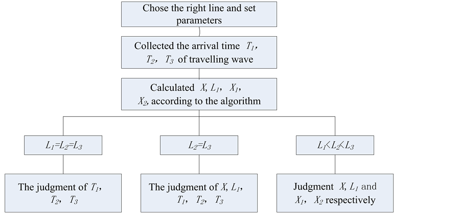
Figure 2. The algorithm simulation process.

Table 1. The line length is AT = L1 = 120 km, BT = L2 = 100 km, CT = L3 = 100 km.
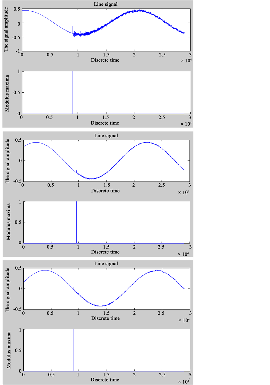
Figure 3. The simulation results of fault in AT, BT, CT.
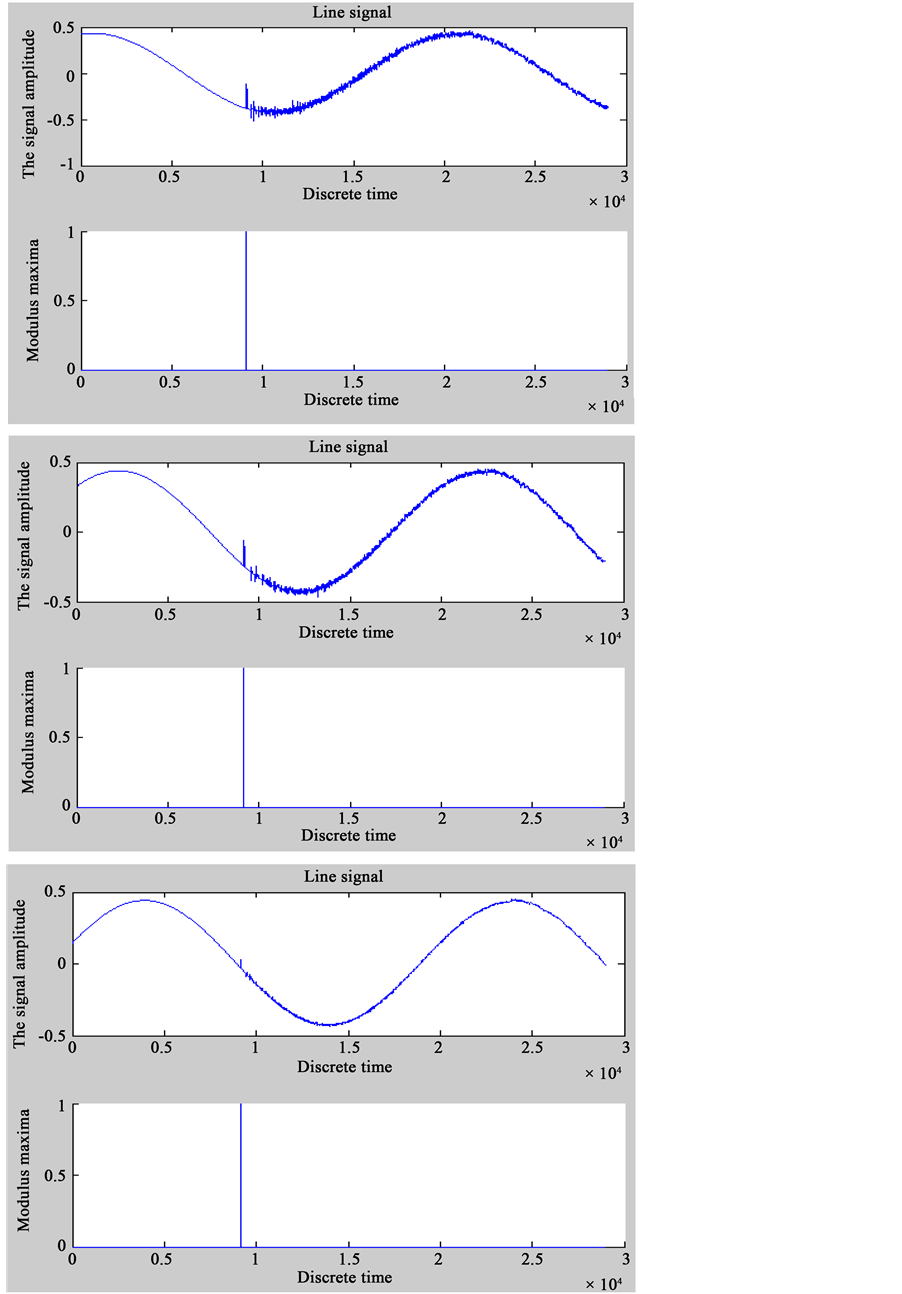
Figure 4. The simulation results of fault in AT, BT, CT.

Figure 5. The simulation results of fault in AT, BT, CT.
Table 2. The line length is AT = L1 = 110 km, BT = L2 = 150 km, CT = L3 = 150 km.
Table 3. The line length is AT = L1 = 120 km, BT = L2 = 150 km, CT = L3 = 200 km.
5.2. The Error Analysis
Analysis by the introduction of traveling wave fault location method decided by two main parameters: one is the arrival time of traveling wave, the other is propagation velocity of traveling wave. The traveling wave propagation velocity is determined by parameters of line. In actual measurement may produce certain error, when find out fault branch and calculate the distance between fault point and end point, it can also produce some small error because of inaccuracy of line measurement. The arrival time of traveling wave caused by sampling precision. Under this paper proposed sampling frequency and the calculation of wave velocity, the resulting error is in the allowable range of engineering.
6. Conclusions
Fault location method based on wavelet transform was propose in this paper. In practical application, we can choose different calculation methods of different line lengths. Traveling wave velocity can be directly determined by parameters of line, while the accuracy of arrival time about voltage traveling wave is improved after wavelet transform; when it had malfunction, the traveling wave arrival time can be obtained and the fault branch can be accurately judged. There is no misjudgment so that the ranging error can meet the needs of practical engineering.
Although this algorithm proved to be feasible by the simulation, it exists limitations in practical application. First, the algorithm is only for T-type transmission network, not for the power transmission system to other networks; second, we should transplant the algorithm to DSP microprocessor to verify the practical feasibility.
Cite this paper
PenggaoWen,HongSong,ZhitingGuo,QuanPan, (2015) Study on Fault Location in the T-Connection Transmission Lines Based on Wavelet Transform. World Journal of Engineering and Technology,03,106-115. doi: 10.4236/wjet.2015.33012
References
- 1. Yu, S.-N., Yang, Y.-H. and Bao, H. (2007) Study on Fault Location in Distribution Network Based on C-Type Travelling-Wave Scheme. RELAY, 35, 1-4.
- 2. Evrenosoglu, C.Y. and Abur, A. (2005) Travelling Wave Based Fault Location for Teed Circuit. IEEE Transactions on Power Delivery, 20, 1115-1121.
- 3. Dong, X.Z., Ge, Y.Z. and Xu, B.Y. (1999) Research of Fault Location Based on Current Travelling Waves. Proceeding of the CSEE, 4, 1-8.
- 4. Qin, J., Chen, X.X. and Zheng, J.C. (1998) Travelling Wave Fault Location Transmission Line Using Wavelet Transform. Proceedings of 1998 International Conference on Power System Technology, Beijing, 18-21 August 1998, 533- 537.
- 5. He, Z.Y. (2008) Application of Wavelet Analysis in the Signal Processing of Power System Transient. China Electric Power Press, Beijing.
- 6. Goudarzi, M., Vahidi, B., Naghizadeh, R.A. and Hosseinian, S.H. (2015) Improved Fault Location Algorithm for Radial Distribution Systems with Discrete and Continuous Wavelet Analysis. International Journal of Electrical Power & Energy Systems, 67, 423-430.
http://dx.doi.org/10.1016/j.ijepes.2014.12.014 - 7. Li, Y.J., Wang, J.S., Zheng, Y.P. and Zhou, W. (2001) Comparison of Several Algorithms of Travelling Wave Based Fault Location. Power System Automation, 25, 36-39.
- 8. Di Santo, S.G. and de Morais Pereira, C.E. (2015) Fault Location Method Applied to Transmission Lines of General Configuration. International Journal of Electrical Power & Energy Systems, 69, 287-294.
http://dx.doi.org/10.1016/j.ijepes.2015.01.014