Theoretical Economics Letters
Vol.4 No.7(2014), Article ID:48478,8 pages
DOI:10.4236/tel.2014.47067
Common Factors in International Bond Returns and a Joint ATSM to Match Them
Christian Gabriel
Faculty of Economics & Business, Martin-Luther University, Halle, Germany
Email: christian.gabriel@wiwi.uni-halle.de
Copyright © 2014 by author and Scientific Research Publishing Inc.
This work is licensed under the Creative Commons Attribution International License (CC BY).
http://creativecommons.org/licenses/by/4.0/


Received 14 April 2014; revised 16 May 2014; accepted 12 June 2014
ABSTRACT
The existence of common factors in international bond markets is an important cause for modelling different term structures of interest rates jointly. This paper investigates the common factors of US and UK treasury yields in the period of 1983 to 2012. A principal component analysis motivates the type of joint ATSM for modelling the yield curves of two distinct economies. In sum, two common factors explain 85% of the yield variation and the model factors have a solid economic intuition.
Keywords:Affine Term Structure Models, Common Factors, Government Bonds, International Term Structure Models, Principal Component Analysis

1. Introduction
Investors are aware of the importance of common factors in international bond markets. If yields across countries depend on each other investing abroad does no longer diversify domestic interest rate risk away. Therefore, international investors immediately benefit from identifying and modeling these factors.
This paper provides an economic analysis of common factors of two major government bond markets. A principal component analysis of US and UK treasury yields in the period of 1983 to 2012 identifies and interprets the factors that drive the international variation. I propose a joint affine term structure model (joint ATSM) to match these factors and study the interaction of empirical and model factors.
[1] applies a principal component analysis to US bond returns and find three factors which correspond to the “level”, “slope” and “curvature” of the yield curve. [2] finds that “level”, “spread” and “steepness” determine a large part of the variation in bond returns from the US, Germany and Japan. [3] studies treasury yields from the US, UK and Germany and concludes that “level” and “slope” govern the most of their variability.
[4] -[6] propose joint ATSM’s to match these common factors in two-currency term structure models. [7] adds an additional risk driving factor to capture the volatility of exchange rate movements. In contrast, [8] -[10] include time variation in the risk premium to cope with the difference in variation of interest rates and exchange rates. [11] provides a classification for completely affine ATSM’s in the [12] sense.
The contribution of the present paper is twofold: Firstly, I provide a factor analysis of US and UK treasury yields in the period of 1983 to 2012. In sum, two common factors explain 85% of the variation of these two major bond markets. I propose a joint ATSM and, to the best of my knowledge, I am the first to provide an economic intuition of the latent factors.
The remainder of the paper is organized as follows: Section 2 provides a factor analysis of the treasury yields. Section 3 proposes a joint ATSM to match the common and local factors. Section 4 links the empirical and model factors and the paper concludes with Section 5.
2. Data
The US and UK zero coupon bonds are provided by the US Federal Reserve and the Bank of England, respectively. The period of 1979 to 1982 is known to be econometrically precarious because of the so called US Federal Reserve experiment [13] . Hence, I investigate the period from January 1983 to July 2012. In line with [1]">1] , I use daily observations of 6-month, 2-, 5- and 10-year treasury yields.
Table 1 reports descriptive statistics of US and UK treasury yields. The average US and UK yield curve is normal (upward sloping) and the short ends are more volatile than the long ends. The correlations within national bond markets are high (ranging from 52% to 95%). The cross country correlations are lower but still significantly positive. These high correlations imply that both yield curves are driven by a limited number of common factors. A principal component analysis provides information on how many factors the yield curve variation is depending [14] . The eigenvalue decomposition in Table 1 shows that a small number of factors describes a large share of the yield curve variation. In sum, two factors account for 85% and four factors for 96% of the yield curve dynamics.

Table 1. Summary statistics.
Means and standard deviations (Std) are reported in p.a. percentage points. Factor analysis is done via eigenvalue decomposition of the yield correlation matrix.
Figure 1 provides insides into the economic interpretation of these factors. The first factor [Common Factor ]">1] has almost the same loading for both countries and all maturities. It is identified as a common factor and interpreted as “level”. For the second factor [Common Factor ]">2] the difference in loading of both countries across all maturities is close to constant. Therefore, I identify it to be the second common factor, interpreted as “spread”. The factor loading of the third factor [Local Factor US] is different for the US and UK term structure. The loadings of the UK yield curve are close to zero. Hence, I identify the third factor to be US specific. Since it is a decreasing function of time to maturity it is interpreted as “slope”. The last plot draws the precisely opposite picture of the fourth factor [Local Factor US]. Whereas US yields play a minor role, the factor loading is a decreasing function of time to maturity of UK yields. Hence, I interpret this local UK factor as “slope”1. The factor analysis leads to the conclusion that the yield curve variation corresponds to two common factors and one local factor each.
3. Model of the Joint Term Structure
Significant improvements have been made in modeling single term structures for pricing
bonds, interest rate derivatives and bond portfolios2. Two country models
are a significant extension of single country models in jointly modeling the dynamics
of term structures of interest rates. The previous section suggests that two common
factors and one local factor each match the variation in US and UK treasury yields
best. That is an
 model of the joint term structure in the
[12] sense.
model of the joint term structure in the
[12] sense.
I follow [11] [12]
in defining the price of a zero coupon bond. Let two economies be described by the
probability space
 where
where
 denotes the physical measure.
 and
and
 shall be the equivalent martingale
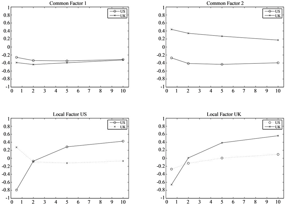
Figure 1. Factor analysis. Factor loadings for US and UK yield curves. A principal component analysis is applied to changes of yields of 6 months, 2, 5 and 10 years time to maturity.
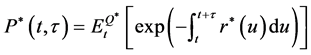
measures for the US and UK, respectively3. In the absence of arbitrage,
the time- prices of an US and UK zero-coupon bond that matures at

 and
and
 are given by
 (1)
(1)
and
 . (2)
. (2)
where
 and
and
 denote
 conditional expectations under
 and
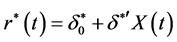
and . A joint ATSM is obtained under the assumption
that the instantaneous short rates
. A joint ATSM is obtained under the assumption
that the instantaneous short rates
 and
and
 are affine functions of a vector of latent state variables
 :
:
 (3)
(3)
and
 . (4)
. (4)
In Equations (3) and (4)
 and
and
 are scalars and
 and
and
 are
are
 vectors.
 nests the local and common factors that drive both
economies. Common factors enter both expressions of
nests the local and common factors that drive both
economies. Common factors enter both expressions of
 and
and
 through non zero
 and
and . Furthermore, the weighting of the factors for
the specific country is expressed in the value of
. Furthermore, the weighting of the factors for
the specific country is expressed in the value of . If
. If
 tends to zero for the common factor, the dynamics of the short rate are (almost)
exclusively driven by the local factor. If, in contrast,
tends to zero for the common factor, the dynamics of the short rate are (almost)
exclusively driven by the local factor. If, in contrast,
 is equally weighted for both countries, there is
a common factor that drives the dynamics of both economies. This has important implications
for international investors. If the short rates share risk factors investing abroad
does no longer diversify domestic interest rate risk away. Hence, it is important
to account for them in the model.
is equally weighted for both countries, there is
a common factor that drives the dynamics of both economies. This has important implications
for international investors. If the short rates share risk factors investing abroad
does no longer diversify domestic interest rate risk away. Hence, it is important
to account for them in the model.
The local factors are forced to be mutually independent, since they would not be
local otherwise. However, they may depend on each other through the correlated common
factors. The one joint ATSM can be decomposed in two single ATSM’s if the local
factors are mutually independent [11]
. The joint dynamics of
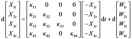
 follow a Gaussian affine diffusion of the form:
 (5)
(5)
 is a 4-dimensional independent standard Brownian
motion under
is a 4-dimensional independent standard Brownian
motion under
 and
and
 and
and
 are
are
 parameter matrices, and
 and
and
 are
are
 parameter vectors. i.e.
 is the level of mean reversion. The paper aims to
provide an economic intuition of the model factors. Therefore, I define the risk
premium to be non time-varying and use a completely affine Gaussian setup4.
The domestic risk premium for US bonds is defined as
is the level of mean reversion. The paper aims to
provide an economic intuition of the model factors. Therefore, I define the risk
premium to be non time-varying and use a completely affine Gaussian setup4.
The domestic risk premium for US bonds is defined as , where
 is a
is a
 parameter vector. The risk premium is country-specific and independent from the
foreign risk premium, i.e. the risk premium parameter of the foreign factor is zero.
Likewise, the UK risk premium is defined as
parameter vector. The risk premium is country-specific and independent from the
foreign risk premium, i.e. the risk premium parameter of the foreign factor is zero.
Likewise, the UK risk premium is defined as , where
 is a
is a
 parameter vector.
So far the model describes the joint dynamics of both term structures of interest
rates. I can also model the country specific dynamics of each country, separately.
Under the risk neutral measure
 and
and
 the affine diffusion
 of the US and UK read, respectively:
 (6)
(6)
and
 . (7)
. (7)
 ,
,
 ,
,
 and
and
 represent the risk neutral measure. Having outlined the short rates
 and
and
 and the underlying diffusion processes
 , I can now turn to the zero bond
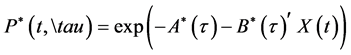
prices. Under the risk-neutral measure
, I can now turn to the zero bond
prices. Under the risk-neutral measure
 and
and
 the price of an US and UK zero-coupon bond read
 (8)
(8)
 (9)
(9)
where ,
,
 ,
,
 and
and
 satisfy ordinary differential equations (ODEs) with the usual boundary conditions
[12]
. The solutions to the ODEs for the process
satisfy ordinary differential equations (ODEs) with the usual boundary conditions
[12]
. The solutions to the ODEs for the process
 are available in closed form.
 and
and
 correspond to the yield data that has been presented in Section 2. [17] give a very practical closed form solution for US (UK)
zero coupon bonds in vector notation.
correspond to the yield data that has been presented in Section 2. [17] give a very practical closed form solution for US (UK)
zero coupon bonds in vector notation.
 (10)
(10)
 (11)
(11)
where
 and
and
 equal
equal
 (12)
(12)
 . (13)
 ,
,
 are functions of
 ,
,
 ,
,
 ,
,
 ,
,
 and the risk neutral and physical parameters correspond
in the following way:
and the risk neutral and physical parameters correspond
in the following way:
 (14)
(14)
 . (15)
To avoid over-identification, I follow the restrictions of
[12] . To that
end I restrict
 to be lower triangle and
 to be the identity matrix. Under the physical measure the diffusion process is given
by:
to be the identity matrix. Under the physical measure the diffusion process is given
by:
 . (16)
Without loss of generality
 and
and
 are assumed to be the common factors.
 is the US local factor and
 is the UK local factor. As both local factors are required to be mutually independent
 .
.
4. Yield and Model Factors
Section 2 has shown that two common factors and one local factor each describe the variation in US and UK treasury bonds best. The corresponding joint ATSM has been presented in Section 3. The following section studies the interaction of yield and model factors. Since my model relies on a completely affine Gaussian setup, I follow [18] in using Kalman filtering with a straightforward direct maximum likelihood estimation. All maturities are observed with a certain error (see [19] [20] ).
Table 2 reports the parameter estimation results.
Each standard error is given in parenthesis. The first panel reports the model parameters.
 are the short rate constants.
 indicate factor specific parameters. Note that the
local parameters US (UK) are set to zero with no standard error for
indicate factor specific parameters. Note that the
local parameters US (UK) are set to zero with no standard error for

 . The model estimates equally rely on the common
factors with values from 0.0097
. The model estimates equally rely on the common
factors with values from 0.0097
 to 0.0133
 and the local
Table 2 . 4-factor joint TSM parameter estimates.
The table reports the estimation results from the four-factor joint ATSM. The estimation is done using daily US and UK treasury yield data from January 1983 to July 2012. I report the parameter estimates and the standard errors in parentheses. A * indicates parameters for the UK market. ε is the standard deviation of observational error associated with the 6 months, 2-, 5- and 10-Years treasury yields from the US and the UK. All other coefficients for the model are described in the text.
factors with values from 0.0103
 to 0.0136
 .
.
 defines the factor dependence structure of the joint
ATSM and each parameter κ is the same for both countries. Yet, the local factors
defines the factor dependence structure of the joint
ATSM and each parameter κ is the same for both countries. Yet, the local factors
 are mutually independent and the factor dependence is set to zero
 . In the last panel the standard
deviation of the observational error is reported. The model matches the data well.
I obtain the biggest observational error for 10 year UK treasury yields with
. In the last panel the standard
deviation of the observational error is reported. The model matches the data well.
I obtain the biggest observational error for 10 year UK treasury yields with .
.
For a standard three factor ATSM there is consensus in the literature to interpret the first three factors as “level”, “slope” and “curvature” (see [1] [18] [21] et al.). However, the case is a little more precarious in the present multi country model. The fitted common and local factors and treasury yields are reported in Figure 2. The first common factor is fitted to the “level” of US treasury yields. The second common factor is fitted to the spread of US and UK 5 year treasury yields in the second graph. These two common factors will explain the common movements of both economies, which correspond to 85% of the overall variation (see Table 1). The variation in yields that can not be explained by the common factors will be explained by the local factors. The local factor US is fitted to the “slope” of US yields which equals the spread of the 10 year treasury yield minus the 6 months treasury yield. The last graph of Figure 2 fits the local factor UK to the “slope” of UK yields. This is the variation in the UK data that can not be matched by the common factors. The local factors explain additional 11% of the total yield variation. All factors exhibit a very high correlation (i.e. up to 0.9848 for Common factor 1 vs “level”) to their economic intuition. These findings are line with [2] [3] . [2] find that “level” and “spread” are common factors whereas the “slope” factor is country specific.
Figure 2 shows that common and local factors are not only an empirical phenomenon. Joint ATSM’s perfectly match the variation of international yields. Furthermore, the latent factors of the joint ATSM gain economic intuition which can be interpreted as “level”, “spread” and “slope”.
5. Conclusion
Investors are aware of the importance of common factors in international bond returns. However, little is known about the linkage and economic interpretation of latent factors of joint ATSM’s. In this paper, I have tried to close that gap and provided a comprehensive study of common factors in US and UK treasury yields. In sum, two common factors already explain 85% of the yield variation of both markets. I propose a joint ATSM and provide a solid economic intuition of the model factors. The two common factors can be interpreted as “level” and
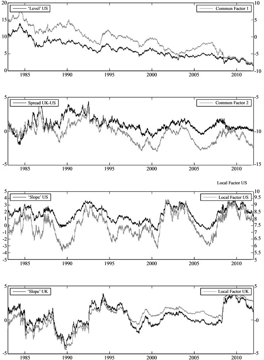
Figure 2. Fitted factors in the four-factor joint ATSM and US and UK Treasury yields. The figure shows the local and common factors of the estimated joint ATSM. Each factor is plotted with its corresponding treasury yield. The first common factor is fitted to the “level” of US treasury yields (10 year US treasury bond). The second common factor and the spread between the 5 year US and UK treasury yields are plotted in the second graph. The third graph shows the local factor US and the slope of the US treasury yields (10 year - 6 months). The last graph shows the local factor UK and the slope of the US treasury yields. Factors and treasury yields run from the 2nd of January 1983 to the 31st of July 2012.
“spread”. In contrast, the “slope” factor is country specific and corresponds to the local factors in the joint ATSM.
Acknowledgements
I am grateful for comments from the brown bag series at Monash University, the participants at the workshops at EFMA Reading and WFC Cyprus, and Philip Gharghori, Jörg Laitenberger and Paul Lajbcygier. All remaining errors are mine, of course.
References
- Litterman, R.B. and Scheinkman, J. (1991) Common Factors Affecting Bond Returns. Journal of Fixed Income, 1, 54-61. http://dx.doi.org/10.3905/jfi.1991.692347
- Driessen, J., Melenberg, B. and Nijman, T. (2003) Common Factors in International Bond Returns. Journal of International Money and Finance, 22, 629-656. http://dx.doi.org/10.1016/S0261-5606(03)00046-9
- Juneja, J. (2012) Common
Factors, Principal Components Analysis, and the Term Structure of Interest Rates.
International Review of Financial Analysis, 24, 48-56.
http://dx.doi.org/10.1016/j.irfa.2012.07.004 - Backus, D., Foresi, S. and Telmer, C. (2001) Affine Term Structure Models and the Forward Premium Anomaly. Journal of Finance, 56, 279-304. http://dx.doi.org/10.1111/0022-1082.00325
- Bansal, R. (1997) An Exploration of the forward Premium Puzzle in Currency Markets. Review of Financial Studies, 10, 369-403. http://dx.doi.org/10.1093/rfs/10.2.369
- Hodrick, R. and Vassalou, M. (2002) Do We Need Multi-Country Models to Explain Exchange Rate and Interest Rate and Bond Return Dynamics? Journal of Economic Dynamics and Control, 26, 1275-1299. http://dx.doi.org/10.1016/S0165-1889(01)00048-3
- Dewachter, H. and Maes, K. (2001) An Admissible Affine Model for Joint Term Structure Dynamics of Interest Rates. Working Paper, KULeuven, Leuven.
- Brennan, M. and Xia, Y. (2006) International Capital Markets and Foreign Exchange Risk. Review of Financial Studies, 19, 753-795. http://dx.doi.org/10.1093/rfs/hhj029
- Sarno, L., Schneider, P. and Wagner, C. (2012) Properties of Foreign Exchange Risk Premiums. Journal of Financial Economics, 105, 279-310. http://dx.doi.org/10.1016/j.jfineco.2012.01.005
- Graveline, J.J. and Joslin, S. (2011) G10 Swap and Exchange Rates. Working Paper, University of Minnesota, Minnesota.
-
Egorov, A., Li, H.T. and Ng, D. (2011) A Tale of Two Yield Curves: Modeling the
Joint Term Structure of Dollar and Euro Interest Rates. Journal of Econometrics,
162, 55-70.
http://dx.doi.org/10.1016/j.jeconom.2009.10.010 - Dai, Q. and Singleton, K.J. (2000) Specification Analysis of Affine Term Structure Models. Journal of Finance, 55, 1943-1978. http://dx.doi.org/10.1111/0022-1082.00278
- Chapman, D.A. and Pearson, N.D. (2001) Recent Advances in Estimating Term-Structure Models. Financial Analysts Journal, 57, 77-95. http://dx.doi.org/10.2469/faj.v57.n4.2467
- Bliss, R.R. (1997) Movements in the Term Structure of Interest Rates. Economic Review, 82, 16-33.
- Dai, Q. and Singleton, K. (2003) Term Structure Dynamics in Theory and Reality. Review of Financial Studies, 16, 631-678. http://dx.doi.org/10.1093/rfs/hhg010
- Feldhütter, P., Larsen, L.S., Munk, C. and Trolle, A.B. (2012) Keep It Simple: Dynamic Bond Portfolios under Parameter Uncertainty. Working Paper, London Business School, London.
- Kim, D.H. and Orphanides, A. (2005) Term Structure Estimation with Survey Data on Interest Rate Forecasts. Finance and Economics Discussion Series Divisions of Research and Statistics and Monetary Affairs Federal Reserve Board, Washington DC.
- Babbs, S.H. and Nowman, K.B. (1999) Kalman Filtering of Generalized Vasicek Term Structure Models. Journal of Financial and Quantitative Analysis, 34, 115-130. http://dx.doi.org/10.2307/2676248
- Duan, J.C. and Simonato, J.G. (1999) Estimating
and Testing Exponential-Affine Term Structure Models by Kalman Filter. Review of
Quantitative Finance and Accounting, 13, 111-135.
http://dx.doi.org/10.1023/A:1008304625054 - Geyer, A. and Pichler, S. (1997) A State-Space Approach to Estimate and Test Multifactor Cox-Ingersoll-Ross Models of the Term Structure. University of Vienna, Vienna.
- DeJong, F. (2000) Time Series and Cross-Section Information in Affine Term-Structure Models. Journal of Business & Economic Statistics, 18, 300-314. http://dx.doi.org/10.2307/1392263
NOTES

1The economic interpretation of the factors of international term structure models as “level”, “spread” and “slope” is in line with . find that “level” and “spread” are highly correlated across countries whereas the “slope” factor is country specific.
2See for literature reviews.

3In the following a * shall indicate the foreign economy.
4 argue that investors even prefer simple (completely affine) to more complex (essentially affine) models.