Journal of Mathematical Finance
Vol.4 No.1(2014), Article ID:42221,12 pages DOI:10.4236/jmf.2014.41004
Applying the Barycentric Jacobi Spectral Method to Price Options with Transaction Costs in a Fractional Black-Scholes Framework
Department of Mathematics and Applied Mathematics, University of Pretoria, Pretoria, Republic of South Africa
Email: eben.mare@up.ac.za
Received October 28, 2013; revised November 30, 2013; accepted December 12, 2013
ABSTRACT
The aim of this paper is to show how options with transaction costs under fractional, mixed Brownian-fractional, and subdiffusive fractional Black-Scholes models can be efficiently computed by using the barycentric Jacobi spectral method. The reliability of the barycentric Jacobi spectral method for space (asset) direction discretization is demonstrated by solving partial differential equations (PDEs) arising from pricing European options with transaction costs under these models. The discretization of these PDEs in time relies on the implicit Runge-Kutta Radau IIA method. We conducted various numerical experiments and compared our numerical results with existing analytical solutions. It was found that the proposed method is efficient, highly accurate and reliable, and is an alternative to some existing numerical methods for pricing financial options.
Keywords:Jacobi Spectral Method; European Options; Fractional Black-Scholes Model; Mixed Brownian-Fractional Brownian Black-Scholes Model; Transaction Cost; Subdiffusive Fractional Black-Scholes Model; Scaling
1. Introduction
Modeling of financial derivatives has been of great interest in the past three decades. Numerous mathematical models have been developed from the classical Black-Scholes [1] framework to help investors in their decision making process. These models are based on an arbitrage argument, i.e., by continuously adjusting a portfolio consisting of a stock and a risk-free bond, an investor can exactly replicate the return to any option on the stock.
In the presence of transaction costs in capital markets, the presence of an arbitrage argument [2] is no longer valid [3], since perfect hedging is impossible. Due to the infinite variation of the geometric Brownian motion, the continuous replication policy incurs an infinite amount of transaction costs over any trading interval no matter how small it might be. Therefore, in recent years, one observes many generalizations of the Black-Scholes model to deal with the problem of option pricing and hedging with transaction costs. This leads to the Black-Scholes model but with an adjusted volatility. Leland [3] was the first to examine option replication in a discrete time setting, and proposed a modified replicating strategy, which depended upon the level of transaction costs, the revision interval, the option to be replicated and the environment. Subsequently, several authors proposed new models, but all in discrete time [4,5]. However, these models based on the diffusion process known as geometric Brownian motion (GBM) have severe shortcomings, for example, long-range correlations, heavy-tailed and skewed marginal distributions, lack of scale invariance and periods of constant values, to enumerate these only. Recently, Wang [6] obtained a European call option pricing formula using a mean self-financing delta hedging argument in a discrete time setting and then showed how scaling and long-range dependence impacted dramatically on the pricing of options using the fractional and multifractional Black-Scholes model with transaction costs.
In continuous time, a lot of efforts have been done in order to alleviate the problem of an infinite amount of transaction costs over any trading interval when the asset process follows a geometric Brownian motion. Magdziarz [7] et al. introduced a subdiffusive geometric Brownian process which captures the subdiffusive characteristics of financial markets. They showed that their model is arbitrage-free. The same idea was used later by Wang et al. [8], Hui and Yun-Xiu [9] to obtain a Black-Scholes equation with transaction costs in subdiffusive fractional Brownian motion regime. However, closed-form solutions of these PDEs in finance are generally rare. Therefore, one has to consider numerical methods to obtain solutions.
In this paper, we are concerned with the application of the barycentric Jacobi interpolation to value options with transaction costs under fractional [6], mixed Brownian-fractional [10] and subdiffusive fractional [8] Black-Scholes models. Barycentric spectral methods were introduced by Baltensperger et al. [11] to solve boundary value problems. Recently, these methods have emerged in the field of finance as a promising tool to solve option pricing problems. Pindza and Patidar [12] proposed an accurate method, namely the barycentric Chebyshev spectral method, to price options in illiquid markets. Ngounda et al. [13] used the barycentric Chebyshev domain decomposition method to provide fast and accurate results for pricing European options with jumps, which was later extended and applied to Heston’s volatility model (see [14]). Most of the work on barycentric spectral methods has been based on the use of uniform or Chebyshev grids. Recently, Wang et al. [15] computed explicit barycentric weights for Jacobi polynomial interpolation in the roots or extrema of classical orthogonal polynomials in terms of the nodes and weights of the corresponding Gaussian quadrature rule. Hence, we investigate the utility of this new barycentric interpolation in the field of finance. The semi-discretization of the PDE in time is realized by using a 7-stage 13th-order fully implicit Runge-Kutta Radau IIA method with adaptive time stepping [16].
This paper is structured as follows. Section 2 reviews the option pricing formulation with transaction costs under fractional, mixed Brownian-fractional and subdiffusive fractional processes. In Section 3, we introduce the Jacobi barycentric spectral method, semi-discretize the PDE in the asset space and propose a conformal map in order to improve the accuracy of our method. In Section 4, we perform numerous experiments in order to advocate the utility of the barycentric spectral method. Finally, Section 5 gives a summary and scope for further research.
2. Pricing with Transaction Costs under Fractional, Mixed Brownian-Fractional and Subdiffusive Fractional Processes
Let  be a complete probability space carrying a fractional Brownian motion
  with Hurst exponent
 , where
  is the set of all possible outcomes of the experiment known as the sample space,
  is the set of all events,
  is a real world probality,
  is a natural filtration,
  a risky underlying asset price process. Assume that the price
  of the underlying stock at time
  satisfies a fractional Black-Scholes model
 (1)
(1)
where ,
,  and
and  are constants. Assume that the portfolio is revised every small fixed time step
 ; transaction costs are proportional to the value of the transaction in the underlying. Let
  denote the round trip transaction cost per unit dollar of transaction. Then under all the assumptions given by Wang [6], the Black-Scholes equation with transaction costs assuming factional Brownian motion can be written as
 (2)
(2)
where the modified volatility is given by
 (3)
(3)
Here  is the fractional Leland number [6].
If we assume that the price  of the underlying stock at time
  satisfies a mixed Brownian-fractional Brownian model
 (4)
(4)
then under all the assumptions given by Wang [10], the Black-Scholes equation with transaction costs in mixed Brownian-fractional Brownian motion can be written as
 (5)
(5)
where the modified volatility is given by
 (6)
(6)
with

A subdiffusive fractional Brownian motion is described by
 (7)
(7)
Wang et al. [8] obtained the modified volatility corresponding to the continuous Black-Scholes equation with transaction cost in subdiffusive regime as
 (8)
(8)
where the modified volatility is given by
 (9)
(9)
Here  represents the gamma function evaluated at
  and
and  is the second derivative of the option value with respect to the asset.
The difference between American and European call and put options is made by the initial and boundary conditions. In this work we focus exclusively on the European call option. Such options have the following initial and boundary conditions
 (10)
(10)
where  and
and . We want to solve the three PDEs (2), (5) and (8) subjected to modified volatilities (3), (6) and (9), respectively. Before moving to the applications of the barycentric Jacobi spectral method to solve these problems, it is worthwhile to consider some preliminaries of this method.
3. Barycentric Jacobi Spectral Collocation Method
In this section, we turn our attention to the problem of barycentric Jacobi interpolation and present a fast algorithm for the efficient computation of the interpolation formula using Jacobi-Gauss-Lobatto (JGL) points. This interpolation is realized by a class of the Lagrange form of the interpolating polynomial, as follows. Let ,
,  be a set of distinct nodes. Then the polynomial of degree
  that interpolates the function
  at these points is given by [17]
 (11)
(11)
where the Lagrange polynomial  corresponding to the node
  has the property
 (12)
(12)
with  Generally, the Lagrange form of the interpolating polynomial (11) is not advocated for numerical computations. In particular, it requires
  additions and multiplications for each evaluation of
  and every time a node
  is modified or added, all Lagrange fundamental polynomials have to be recalculated. However, with slight modifications, the Lagrange formula is indeed of great practical use. This has been noted by several authors, including Henrici [18] and Werner [19]. Berrut and Trefethen [20] modified the Lagrange polynomial through barycentric interpolation and proposed an improved Lagrange formula. Following [20], we define
 , the numerator of
  in (11) divided by
 , as
, as
 (13)
(13)
In addition, if we define the barycentric weight by
 (14)
(14)
i.e.,  , then
  in (11) becomes
 (15)
(15)
Consequently, the Lagrange formula (11) becomes
 (16)
(16)
In particular, if , we obtain
 (17)
(17)
Dividing (16) by (17), we get the barycentric formula for  as
as
 (18)
(18)
This is the most used form of Lagrange interpolation in practice and admits  operations. In order to obtain good approximations via interpolation, the choice of interpolation nodes and barycentric weights is particularly important. For certain particular sets of points, such as equidistant points as well as Chebyshev points, the barycentric weights
  can be computed analytically [20]. Recently, Wang et al. [15] computed explicit barycentric weights for polynomial interpolation in the roots or extrema of classical orthogonal polynomials in terms of the nodes and weights of the corresponding Gaussian quadrature rule.
In this paper, we are interested in the barycentric Jacobi interpolation. The Jacobi-Gauss-Lobatto quadrature rule is defined by
 (19)
(19)
where the Jacobi-Gauss-Lobatto points  are the zeros of
  and
and  is the Jacobi polynomial of degree
 . The following result gives an analytical formula of barycentric weights for the Jacobi-Gauss-Lobatto points.
Theorem 3.1 ([15]) Let , be the roots of
  and let
  be the corresponding weights of the interpolatory quadrature rule with weight function
 . Then the simplified barycentric weights are for Jacobi-Gauss-Lobatto points, the simplified barycentric weights
  are given by
 (20)
(20)
The proof of Theorem 3.1 can be found in [15].
The computation of entries of the first and second order differentiation matrices  and
and  where
where
 (21)
(21)
is given as in [11] by
 (22)
(22)
 (23)
(23)
where .
.
3.1. Conformal Mappings for High Resolution of Non-Smooth Initial Conditions
It is well-known that the solution of Equation (8) is very sensitive to localization errors when  is in the vicinity of
 , because the second derivative of the payoff does not exist at this point. Therefore, to increase accuracy it would be reasonable to use an adaptive mesh with high concentration of the mesh points around
 , while a rarefied mesh could be used far away from this area. If we assume that
 , where both
  and
and  are finite, then without further loss of generality we may assume that the interval of integration is
 , as the linear transformation
 (24)
(24)
In this paper, we use the conformal map  given in [21] by
 (25)
(25)
where
 (26)
(26)
with
 (27)
(27)
where  and
and  determine the magnitude of the region of rapid change and the location, respectively. Here,
  represents the Jacobi-Gauss-Lobatto points.
In Figure 1, we plot the new grid obtained from the original Jacobi  grid by using transformations (25) and (24) together. The new grid in
  contains 100 nodes distributed from
  to
to . Value of parameters used in this example are:
  and
and , where
  is the strike price. In addition, we show the transformation function around
  for
for  (black),
  (green),
  (purple) and
  (red). We observe that when
  decreases the grid approaches a Jacobi-Gauss-Lobatto

Figure 1. Asset direction grids S obtained from the mapped Jacobi grids x.
grid distribution one. When  increases we accommodate more grid points around the strike price.
A significant advantage of the barycentric Jacobi spectral method is that it eliminates tedious computations of transformed derivatives using the chain rule as is usually the case in other spectral collocation methods.
3.2. Application to the Black-Scholes PDE
We discretize the Black-Scholes PDEs (2), (5) and (8) in the asset (space) direction by means of barycentric Jacobi spectral method. Let  be the transformed Jacobi-Gauss-Lobatto points, the first step is to transform
  into
into  that better suits the option at hand using
  Now writing
 , the PDE (8) together with its initial and boundary conditions yields
 (28)
(28)
where

Substituting (11) into (28) yields the following system of nonlinear ODEs
 (29)
(29)
In order to write (29) in matrix form, we introduce the following matrix and vector notations
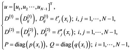 (30)
(30)
where  is an
is an  identity matrix. Consequently, (29) can be expressed as an initial value problem of the form
 (31)
(31)
where
 (32)
(32)
We use a 7-stage 13th-order fully implicit Runge-Kutta Radau IIA method with step size control to integrate the system of ODEs (31). The method is B-stable and stiffly accurate. Details of the method can be found in [16].
4. Numerical Results and Discussions
We apply the barycentric Jacobi spectral method to value Black-Scholes equations with transaction costs under fractional (FBS), mixed Brownian-fractional (MBS) and subdiffusive fractional (SBS) processes. To show the efficiency of the present method we report the root mean square norm error  of the solution computed with
  grid points, given by
 (33)
(33)
and the maximal norm error 
 (34)
(34)
where  and
and  are the benchmark and computed values of the solution
  at
at .
.
The analytic solutions of Black-Scholes equations with transaction costs under FBS, MBS and SBS regime are possible if we assume that the Greek  is always positive for the above mentioned models as in the case of standard Black-Scholes model, then for European call options under SBS [6] regime is known, and expressed as
 (35)
(35)
where
 (36)
(36)
here  is given by
 (37)
(37)
 and
and  is the cumulative probability distribution function for a standardized normal variable
 (38)
(38)
If we assume the same sign behaviour for  in the MBS model, then the analytic solution is given by
 (39)
(39)
where
 (40)
(40)
with the modified volatility given by
 (41)
(41)
Here  and
and . In the case of FBS model, the closed-form solution is given as
 (42)
(42)
where
 (43)
(43)
with
 (44)
(44)
In order to test the accuracy of the method, we present a comparison against the above exact solutions. In Figure 2 (top left) we plot together numerical and exact solutions for comparison purposes. We select numerical values of the parameters to be ,
,  ,
,  ,
,  ,
,  ,
,  ,
,  ,
,  ,
,  ,
,  ,
, . We choose the tolerance of the 7-stage 13th-order fully implicit RungeKutta Radau IIA method [16] to be
 , so that the error is dominated by the spatial error. Clearly, it is observed that all numerical solutions are in good agreement with exact ones.
To see how good our numerical approach approximates exact solutions, we plot the absolute error, i.e., absolute distance between the exact solution and the numerical approximation for all three models. This shows very good accuracy for our method.
4.1. Effect of Changes in N and Smax
To determine the convergence of the discretization scheme, we solve the problem by keeping some parameters fixed and varying others. We fist investigate the effect of the truncation domain on the errors by varying  between 120 and 500 and keeping other parameters fixed as
 ,
,  ,
,  ,
,  ,
,  ,
,  ,
,  ,
,  ,
,  ,
,  and
and . Figure 3 show the
  -norm and
  -norm errors, respectively. We notice that the errors remain bounded and do not vary significantly in term of the truncation domain. This is an important result, since we can accurately solve the option pricing problem on a small truncated domain, which will result in better efficiency.
In the next experiment, we investigate the convergence of the barycentric Jacobi spectral method. We vary the number of collocation points  between 20 and 300, with parameters
 ,
,  ,
,  ,
,  ,
,  ,
,  ,
,  ,
,  ,
,  ,
,  ,
, ; and we plot the results in Figure 4 (top left and right).
For all three models, our method converges rapidly to the exact solutions. This is usually known as spectral or exponential convergence. The efficiency of our approach is measured in Figure 4 (bottom left and right) by the CPU time. The results on the efficiency of our method are very satisfactory for all three methods. An accuracy of  can be obtained in less than a second.
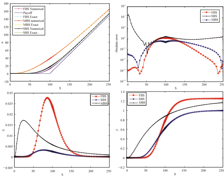
Figure 2. Solutions of the European call options with transaction costs under the three models (top left), absolute error (top right), the Delta (bottom left) and Gamma (bottom right) of the three models with ,
,  ,
,  ,
,  ,
,  ,
,  ,
,  ,
,  ,
,  ,
,  and
and .
.

Figure 3. Effect of the truncation domain on the  -norm and
  -norm in computation of the three models with parameters
 ,
,  ,
,  ,
,  ,
,  ,
,  ,
,  ,
,  ,
,  ,
,  and
and .
.
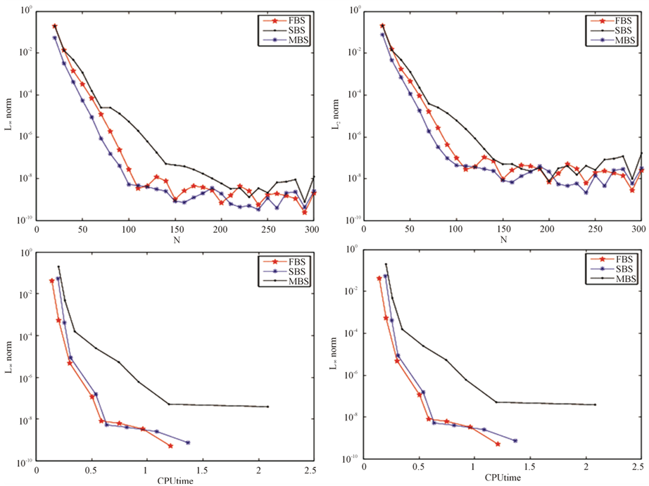
Figure 4. Convergence of  and
and  -norms and efficiency of the barycentric Jacobi spectral method with parameters
 ,
,  ,
,  ,
,  ,
,  ,
, ,
,  ,
,  ,
,  ,
,  and
and .
.
4.2. Convergence of the Method
We explore the effect of changes in time, as well as grid-stretching on the accuracy of the model, keeping

 fixed and allowing
  to vary between
 ,
,  and
and , we compute the
  - and
- and  -norms for
 ,
,  and
and . The results are shown in Table1
We notice that when the grid stretching parameter  increases, the accuracy of our method is improved. By accommodating more grid points around the strike price
 , we can overcome the poor convergence of naive application of numerical methods when pricing options. We also observe that our method is highly accurate (even for long maturity options).
We also explore the effect of changes in time, as well as Jacobi parameters  and
and  on the accuracy of the model, keeping
 ,
, 
 fixed and allowing
  and to vary between
 ,
,  and
and , and
, and  to vary between
 ,
,  and
and , we compute the
  - and
- and  -norms for
 ,
,  and
and . The results are shown in Table2
Once again the barycentric Jacobi spectral method achieves very good accuracy for all three models (even for long term maturity). The Jacobi parameters chosen here do not impact the accuracy of our methodology significantly. It would be useful to investigate how to choose these parameters in an optimal way, however, this is beyond the scope of this paper.
5. Conclusion
The work of Leland [3] on the discrete option pricing model and replication with transaction cost has paved the way to develop the continuous version. We exploited the continuous version by Wang et al. [8] to construct

Table 1 . Norm infinity and norm relative of errors for the European call options with transaction costs under subdiffusive regime (SBS), fractional Brownian (FBS) and multifractional Brownian (MBS) motions.
Table 2. Norm infinity and norm relative of errors for the European call options with transaction costs undersubdiffusive regime (SBS), fractional Brownian (FBS) and multifractional Brownian (MBS) motions.
spectral-based solutions to the model. In practice, option pricing problems are solved numerically since analytical solutions rarely exist. We acknowledge that many studies have been conducted in the domain of finance and both numerical and analytical solutions have been investigated. However, the barycentric Jacobi spectral method has just been proven to have a better accuracy and has not been studied in the field of PDEs in finance. Furthermore, this method obtains solutions with greater accuracy than the usual well-known and studied numerical schemes. The barycentric Jacobi spectral method has full differentiation matrices, which require more computational effort than sparse differentiation matrix methods. In order to improve the efficiency of the rational Jacobi spectral method, we are currently investigating the domain decomposition algorithm which yields block diagonal matrices and we expect to have a greater accuracy, and at least less computational time and memory.
Acknowledgements
This work is supported by the Faculty of Natural and Agricultural Science of the University of Pretoria. B. F. Nteumagne and E. Pindza would like to thank Mr. Brad Welch for his financial support in this research.
REFERENCES
- F. Black and M. Scholes, “Pricing of Options and Corporate Liabilities,” Journal of Political Economy, Vol. 81, No. 3, 1973, pp. 637-654. http://dx.doi.org/10.1086/260062
- J. C. Hull, “Options, Futures and Other Derivatives,” 4th Edition, Prentice-Hall, Upper Saddle River, 2000.
- H. E. Leland, “Option Pricing and Replication with Transaction Costs,” Journal of Finance, Vol. 40, No. 5, 1985, pp. 141-183. http://dx.doi.org/10.1111/j.1540-6261.1985.tb02383.x
- P. Boyle and T. Vorst, “Option Replication in Discrete Time with Transaction Costs,” Journal of Finance, Vol. 47, No. 1, 1992, pp. 271-293. http://dx.doi.org/10.1111/j.1540-6261.1992.tb03986.x
- M. Monoyios, “Option Pricing with Transaction Costs Using a Markov Chain Approximation,” Journal of Economic Dynamics and Control, Vol. 28, No. 5, 2004, pp. 889-913. http://dx.doi.org/10.1016/S0165-1889(03)00059-9
- X. T. Wang, “Scaling and Long-Range Dependence in Option Pricing I: Pricing European Option with Transaction Costs under Fractional Black-Scholes Model,” Physics A, Vol. 389, No. 3, 2010, pp. 438-444. http://dx.doi.org/10.1016/j.physa.2009.09.041
- M. Magdziarz, “Black-Scholes Formula in Subdiffusive Regime,” Journal of Statistical Physics, Vol. 136, No. 3, 2009, pp. 553-564. http://dx.doi.org/10.1007/s10955-009-9791-4
- J. Wang, J. R. Liang, L. J. Lv, W. Y. Qui and F, Y. Ren, “Continuous Time Black-Scholes Equation with Transaction Costs in Subdifusive Fractional Brownian Motion Regime,” Physics A, Vol. 391, No. 3, 2012, pp. 750-759. http://dx.doi.org/10.1016/j.physa.2011.09.008
- H. Gu and Y.-X. Z, “Pricing Option with Transaction Costs under the Subdiffusive Black-Scholes Model” Journal of East China Normal University, Vol. 5, 2012, pp. 85-92.
- X. T. Wang, E. H. Zhu, M. M. Tang and H. G. Yan, “Scaling and Long-Range Dependence in Option Pricing II: Pricing European Option with Transaction Costs under the Mixed Brownian-Fractional Brownian Model,” Physics A, Vol. 389, No. 3, 2010, pp. 445-451. http://dx.doi.org/10.1016/j.physa.2009.09.043
- R. Baltensperger, J. P. Berrut and B. Noël, “Exponential Convergence of a Linear Rational Interpolant between Transformed Chebyshev Points,” Mathematics of Computation, Vol. 68, 1999, pp. 1109-1120. http://dx.doi.org/10.1090/S0025-5718-99-01070-4
- E. Pindza and K. C. Patidar, “Spectral Method for Pricing Options in Illiquid Markets,” Proceedings of the International Conference on Numerical Analysis and Applied Mathematics, Vol. 1479, 2012, pp. 1403-1406.
- E. Ngounda, K. C. Patidar and E. Pindza, “Contour Integral Method for European Options with Jumps,” Communications in Nonlinear Science and Numerical Simulation, Vol. 18, No. 3, 2013, pp. 478-492. http://dx.doi.org/10.1016/j.cnsns.2012.08.003
- E. Ngounda, K. C. Patidar and E. Pindza, “A Robust Spectral Method for Solving Heston’s Volatility Model” Journal of Optimization Theory and Applications, Springer US, 2013.
- H. Wang and D. Huybrechs, “Explicit Barycentric Weights for Polynomial Interpolation in the Roots of Extrema of Classical Orthogonal Polynomials,” Report TW604, Department of Computer Science, Katholieke Universiteit Leuven, 2012.
- E. Hairer and G. Wanner, “Solving Ordinary Differential Equations, II: Stiff and Differential-Algebraic Problems,” PringerVerlag, New York, 1991. http://dx.doi.org/10.1007/978-3-662-09947-6
- J. L. Lagrange, “Leçons Elémentaires sur les Mathématiques, Données à l’Ecole Normale en 1795,” Journal de l’École Polytechnique, Vol. 7, 1795, pp. 183-287.
- P. Henrici, “Essentials of Numerical Analysis with Pocket Calculator Demonstrations,” Wiley, New York, 1982.
- W. Werner, “Polynomial Interpolation: Lagrange versus Newton,” Mathematics of Computation, Vol. 43, 1984, pp. 205-217. http://dx.doi.org/10.1090/S0025-5718-1984-0744931-0
- J. P. Berrut and L. N. Trefethen, “Barycentric Lagrange Interpolation,” SIAM Review, Vol. 46, 2004, pp. 501-517. http://dx.doi.org/10.1137/S0036144502417715
- T. W. Tee and L. N. Trefethen, “A Rational Spectral Collocation Method with Adaptively Transformed Chebyshev Grids Points,” Journal of Scientific Computing, Vol. 28, No. 5, 2006, pp. 1798-1811.