Journal of Mathematical Finance
Vol.3 No.2(2013), Article ID:31814,7 pages DOI:10.4236/jmf.2013.32026
Absolute Adviser or Stochastic Model of Trade on the “Heavy Tails” of Distributions
The National Research Technological University, Moscow, Russia
Email: aleksei-avdeenko@mail.ru
Copyright © 2013 Alexey M. Avdeenko. This is an open access article distributed under the Creative Commons Attribution License, which permits unrestricted use, distribution, and reproduction in any medium, provided the original work is properly cited.
Received January 22, 2013; revised March 24, 2013; accepted April 8, 2013
Keywords: Heavy Tails; Forex Market; Adviser
ABSTRACT
The algorithm of trade on the “heavy tails” of distributions of financial sequences is considered. Critical conditions and parameters for the implementation of win-win adviser are established. The algorithm subjected to the total testing the Forex market for the periods 1990-2012. The material is presented in the maximum available for non-mathematicians form.
1. Introduction
Econometric theory possesses a wide range of standard models. These are models of moving average MA (q), autoregression AR (p), and mixed models, such as ARMA (p, q) [1,2]. These models are incapable of predicting dynamics of conditional dispersion. Next step of approximation is represented by ARCH (q)—type models, where conditional dispersion is treated as linear function of squares of the past anomalies. This approximation was subsequently generalized into the GARCH (p, q) model, where conditional dispersion at a given time is linear function of conditional dispersion and squares of anomalies at previous times [3,4].
It is possible to treat model GARCH (p, q) as ARMA (p, q) process, to determine stationary conditions, and to use it for forecasts of volatility. Next refinement of the GARCH (p, q) model is model EGARCH (p, q) capable of allowing for the asymmetry effects—that is for negative correlation between profitability and volatility.
Mathematical aspects of these models are rather simple, but their actual application to creation of automated trading systems isn’t very efficient. Determination of the model’s coefficients may be implemented in the form of one or another statistical procedure, or with use of neural networks. In this case, however, practical implementation brings about trivial results—the model’s coefficients either aren’t significant in statistical sense, or are determined with accuracy, which does not suffice for efficient decision making, for instance, regarding input into or output from the short or long position.
Author of the proposed article chooses somewhat a different way: to analyze dynamics of conditional probabilities rather than dynamics of conditional moments, and specifically not for all anomalies, but for the socalled “tails” of the distribution—that is significant deviations, whose share is about 10−4 ··· 10−3 of the entire sequence. This algorithm has been embedded into the adaptive behavior model [5-7] and implemented in the MQL-5 media.
А number of the most complex problem are on a joint of the determined and statistical description. Where does determinacy finish and the accounting of statistical properties of system is necessary? A lot of important effects lie out of availability of standard statistical procedures: just rare events, instead of average properties often define the behavior of the system.
Thus it is necessary to make a note that rare events are events nevertheless happening repeatedly, just their share is the total number of events and it is very small. For rare events it is also possible to use statistical techniques, the so-called statistics of the “tails” of the distribution.
2. The Model of the “Tails” of Distributions
Let the background—discrete financial sequence  of the quotation of the currency pair at time tn.
To exclude minor fluctuations (less spread) under the  we will understand the weighted average of the opening price, the closing, the maximum and minimum for a given timeframe, which put equal to the minimum possible
 . Enter the value
  of the change
  in the evolution of the systems.
Value  will be considered as a stochastic process. In the future depending on the convenience will record
  as
as  or
or  and understanding that we always deal with the discrete random variable defined only in a time point tn.
Only one but quite natural assumption concerning process —ergodicity, i.e. equality of an average on trajectories to an average on time.
More difficult to determine the stationary or its nonstationary of the stochastic process . From the formal point of view stationary in narrow sense is an independence of n dimensional density distribution
  from a shift in time
 .
.
Obviously, this is determined by the interval of the consideration of functions: for large intervals, the process is almost stationary, for small, of course, no. In particular, the trend generates nonzero first moment of one-point distribution density, change the sign of the trend— change the moment and as a consequence non-stationary of the process.
It is also need to consider the fact that in any analysis we deal with sample statistics rather than statistics of a population: i.e. really are random moments and histogram of distribution (empirical statistics), but not the required moments and distribution density.
In the future, provided the context of this work under a stationary process we mean indistinguishability distribution functions for time-shift within one or another statistical hypothesis accepted or rejected with a significance level . In particular, it is convenient to use the nonparametric Kolmogorov, which allows you to test two samples {x} {y} belonging to one distribution. For this purpose the maximum difference of two empirical functions of distribution
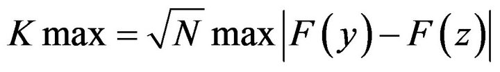 , compared to tabular value is calculated at defined risk level.
In Figure 1 is presented a histogram of the empirical distribution of values for the pair EUR/USD for the period 2012. Total used 120,000 pixels, the histogram has 20 digits, the value  of one minute difference weighted averages for the convenience of reporting estimates, multiplied by 105, expressed in the so-called units “Point”.
Changes to the “past” to any value in the range from 104 to 3 × 10⁵ minutes with a risk level 0.01 by criterion of Kolmogorov didn’t allow to identify a statistically significant difference of empirical distributions. This suggests the stationary of the process, at least in these scales.
The restoration of the theoretical probability density
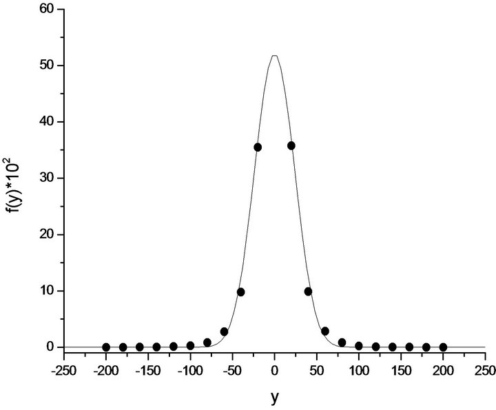
Figure 1. Histogram of distribution (•), y(t) and approximation of the model (1).
can be conducted in different ways. One of the options was used in [5] and is associated with finding the stationary solutions of the Fokker-Planck equation. However, there is a more obvious way, based on the theory proposed by H. Haken and others, the principle of maximum information entropy [8].
According to this principle, in the presence of empirical limitations—moments of order  the stationary probability density has the form
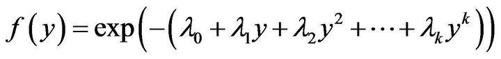 where the
  Lagrange multipliers (the constants of the model in fact) to determine which you can use the method of gradient search (evolutionary strategy).
It is possible to show that the method is reduced to the system of equations if missing simple details.
 (1)
(1)
where  is the average of required functions of distribution, thereby depending on all
 ;
;  an average of the distribution, which is set by the system, i.e. an empirical average,
  a constant which determines the speed of relaxation.
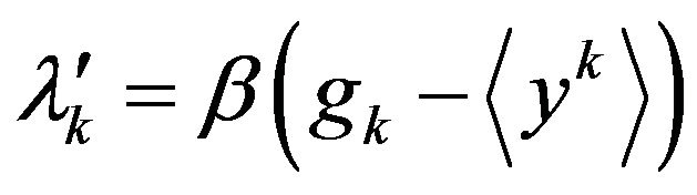
The prime on the size —is derivative of “relaxation time”, the difference between two successive approximations
 . Values
  are determined by numerical integration or by using the perturbation theory, for example in the form of chart equipment, the multiplier
  is determined from the normalization conditions.
It is not difficult to determine a multipoint probability density . In this case, as outer limits, you can use point-to-point correlation functions
 .
.
Much more interest represented by so-called conditional density of distribution, for example, point-to-point conditional density:
This function characterizes joint distribution of random variables , yn if value
  is set. The algorithm is similar to the used above, but in this case, the Lagrange multipliers depend on the value
 .
.
Use the Equation (1), which was constructed of nonGaussian approximation or theoretical distribution of fluctuations of an exchange rate of pair EUR/USD— solid line in Figure 1.
It was chosen the model of an even degree1 of relative not higher than the fourth order, i.e. the outer limits served empirical moments.
The relevant values are ,
,
 . From here, you can evaluate the amplitude of the oscillations with a significantly non-Gaussian component or so-called “heavy tails” of the distributions
 which is approximately amounts 214 units in the system of coordinates or 2.14×10⁻³ in absolute values.
In other words, a decline of more than 0.2 per cent for a minute is connected with the significant non-Gaussian component. This is the “tails” of the probability density, which are significant non-linear effects. However, the absolute share of the “tails” in a sequence is small (5 - 15) × 10–5, or an average of 2 to 5 bursts per month.
Exactly these “tails” of the probability density and its algorithms trading will be considered in the future.
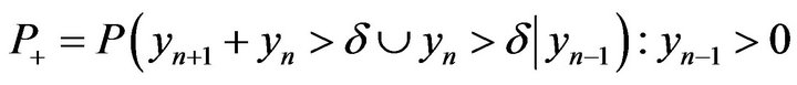
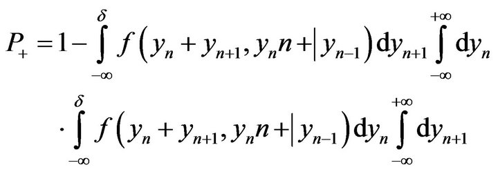
Let —be the trading spread. We introduce the conditional probabilities P + P—in following way:
 ,
,
The meaning of these values is obvious. They are the probability that a given positive or negative races  in time
  jump in the time
  or at the time
  exceed the amount of the spread. If the conditional probabilities
  synthesized with the help of algorithm of (1), the process of calculation is obvious.
For example
In this case, the probability  are the functions of variable
  expressed through the dependencies in the right order of smallness
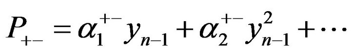 .
.
In Figures 2 and 3 separately various signs  dependences of conditional empirical probabilities P + P—from
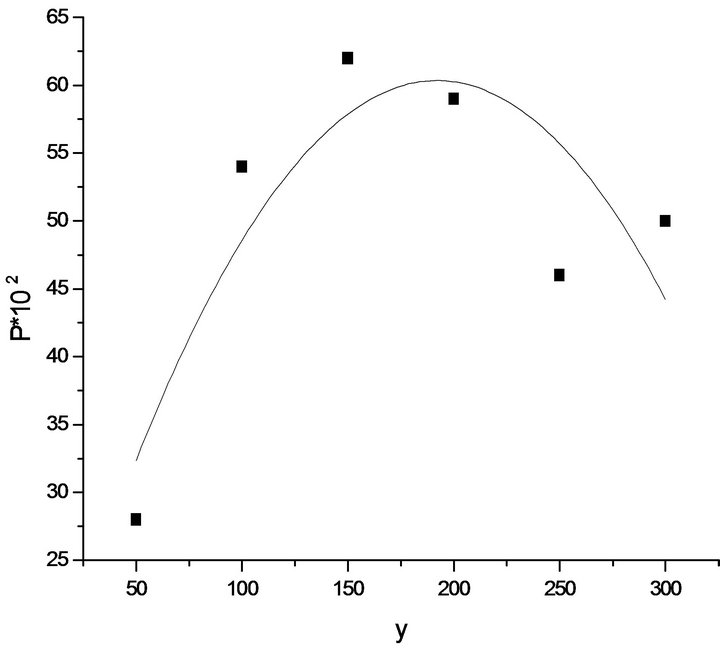
Figure 2. Probability P+ depending on changes y; y > 0; 1 min, EUR/USD, 2012.
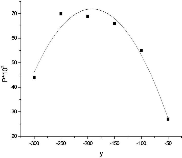
Figure 3. Probability P− depending on changes y; y > 0; 1 min, EUR/USD, 2012.
value —symbols (■) and theoretical approximation by polynomials not exceeded the second order are submitted.
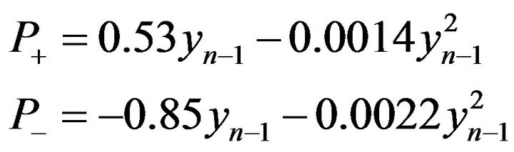 (2)
(2)
Graphs and correlations (2) are of considerable interest to trade on the tails of the distribution. Indeed, if the previous change is small, then the probability that it will keep the sign and exceed spread less than half, with changes over 100 - 120 units, reaches 0.65 ··· 0.70, and finally, with extra-large race again becomes more likely the change of sign. You can make an assessment of the conditions, under which the maximum probability of preserving the direction of movement of the exchange rate 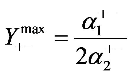 and extra-large amplitude, in which
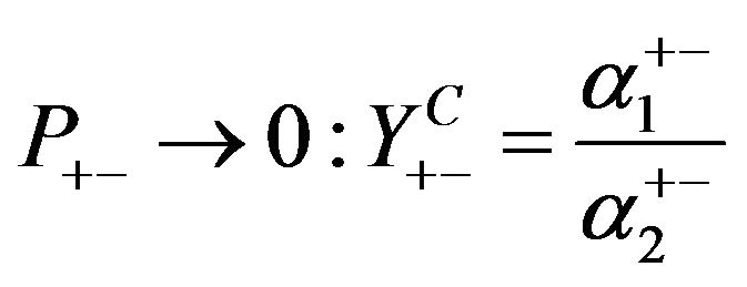 .
.
Corresponding values in the scale are 189 - 193 and 378 - 376 units, respectively, for the positive and negative jumps in the exchange rate. Assessment of the  close to appropriate assessment of the amplitude nonlinear effects is calculated earlier. From here possible evaluation of the profitability of the algorithm trade on their “tails”, it is the excess of the amount of profitable trade for the time
  is:
is: , where
  is the probability of observing jump the maximum
 ,
,  is the maximum value of the conditional probability. Substituting the corresponding values of the histogram and the relations (2), we have
 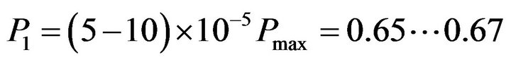 , which corresponds to 1 ··· 3 trade in a month or 12 ··· 36 in a year.
The program block that implements this algorithm in the general scheme is illustrated in Figure 4 in curly brackets. It can function separately from the rest of the algorithm, and together, including the option of a multicurrency trading.
3. Testing of the Algorithm
Trading algorithm on the “tails” of the distribution had been subjected to total testing pair EUR/USD with 1 minute timeframe for various periods of time. Since the measurement of the number of (not probability) successful traders gives the 12 - 36 of trade in the year, there were selected more time testing from six months up to five years or more. The algorithm was tested separately from the other blocks of adaptive behavior shown in Figure 4.
In particular, the five-year interval 1995-2000, twelve years 2000-2012 and five two-year intervals from 2000 to 2008. Besides generating random intervals of 6 months
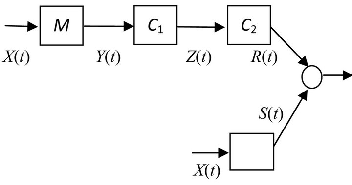
Figure 4. Adaptive behavior algorithm flow chart. Herein M is model, C1,2 are controllers, X(t) is input signal, Y(t) is the estimated future, Z(t)—integrated management of the controllers 1, R(t)—adaptive behavior model decision and S(t)—the solution to the “tails” of the distribution.
from 2000 to 2012. Parts of the results are given in Table 1. Initial balance was $10,000.
Total profit, the number of trade and drawdown at the different levels of risk from 0.05 to 0.10 and from 0.05 up to 0.20 are estimated. In this algorithm, the communication of risk levels with the model was mediated by risk level determined the lot size depending on the success of the previous trading, as a function of the level of free margin, and does not influence the criteria of input—output in the short or long positions.
Not been established by any of the unprofitable period of more than 6 months. Although for periods of two years and more than the maximum drawdown was 20 percent of the final profit. The number of trade ranged from 4 to 22 in a year, which is close to the a priori estimates.
The most effective was the period of 2010-2012. The latter is connected to the fact that for the acceleration test constants were calculated only once for 2012. On the other hand, this is evidence of the sustainability of the suggested algorithm and, most importantly, on the stationary of the process in the scale.
Finally, at the end of the table are submitted the results of testing the expert on the period of 22 years from 1990 to 2012. In the last column in parentheses is indicated the average annual income for different levels of risk. The average of traders in the year is about 10. The profit depending on the level of risk—from amounts from 970% to 10,820% (11.4 and 23.8 per cent per year).
A small number of trades are determined by the same structure of the algorithm and are a consequence of the small number of major (critical) deviations. However, the algorithm unmistakably recognizes the big races, and took, almost always, an adequate solution.
The algorithm is the most preferable for large investors, for which stability is more important profitability.
4. Nonlinear Effects in Other Scales
“Heavy tails” of distribution of changes of quotations of currency pairs exist in all description scales, i.e. at all values of an interval of preliminary smoothing. From the formal point of view it can be shown by means of continual integration on intermediate conditions of integral on trajectories—solutions of the corresponding equation of Fokkera-Planck [3].
However, in applied aspect (a subject of offered article), it is enough to consider conditional probabilities of these or those conditions at a preset value of amplitudes of previous conditions and on this basis to realize amendments to trade strategy.
So, let —deliberately an average with the period of opening, closing, a minimum and a maximum of quotations of the corresponding currency pair since timeframe 1 min. Respectively yn—its change with an
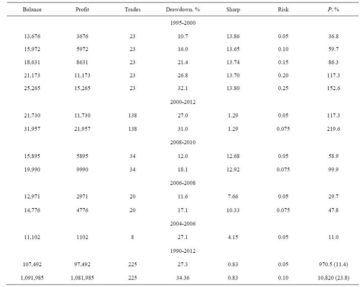
Table 1. Balance, traders, drawdown, Sharpe ratio and the risk for various periods of testing.
interval p1.
Let’s enter conditional probability 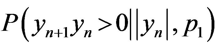 of preservation of a sign of changes at the set previous value of the module and the averaging period p1.
The relevant empirical dependences for EUR/USD pair for the period 2012 at different values are presented in Figure 5.
Value  for ease of presentation at one scale is standardized on empirical variance
 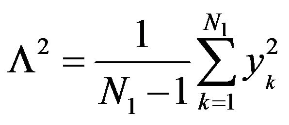 with the step
  on the basis
  of points
 .
.
If the amplitude of the preceding condition is close to 0.5 then the probability preserve the sign is close to half, in other words, both increase and decrease in quotations are equally probable, however, if  then the sign is significantly more likely to preserve (i.e. continuing the trend).
Naturally, with the share of implementations of such a
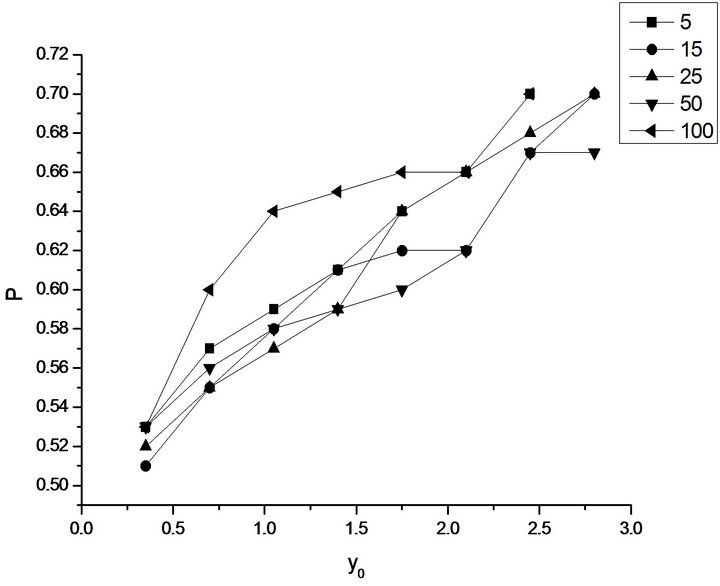
Figure 5. The dependence of the conditional probability of preservation of the sign change of the quotations on the amplitude of the smoothed values for the previous pair EUR/USD at different values for the year 2012.
state decreases sharply and is about 10–4 - 10–3. In the scale of averaging  not found the opposite trend, which took
  place in Figures 2 and 3 and they reduce the probability preserve the sign of the too big size
 .
.
More precisely, in some cases this has been observed for some periods , but the number of implementations of these conditions were too little, even at the annual observation, and therefore does not allow yet to make a statistically significant conclusions.
This result is valid for all sizes averaging and can be considered, apparently, the fundamental law for financial sequences, namely the probability of preserving the sign of changes in financial sequence increases almost linearly with the increase of the amplitude of the previous state  at any intervals preliminary to averaging.
These additional effects were taken into account in the block of the controller of the full model of adaptive behavior Figure 4. In other words, the entrance to the short or long position was determined not only by the adoption of a resolution adaptive behavior in the controller C1, but by condition . The full testing of the algorithm was held at EUR/USD pair for the period 2012. The results are presented in Figure 6.
For ease of presentation of the results the total number of trade has been divided by the maximum value of the variable, which amounted to 21. In addition, it was thought that a lot size is constant L = 3, contrary to the testing of the algorithm only “tails”, in which L was determined on the value of free funds and amounted at an average of 0.5 - 0.8 standard lot in the $100,000. The original balance, as before, was $10,000.
With the growth value , which designated y0 on
Figure 6. Total profit (S), the number of trades (n), and the probability (P) of profitable trades, depending on the amplitude of the preceding state.
the graphics increases the probability of profitable trades is small but decreases the total number, which remains unchanged during , that corresponds to “turn off” the complete algorithm and operation of its part related only to trade on the “tails” with minimal averaging period. Testing of the algorithm, this is reflected in Table 1.
5. Discussion and Prospects
The term “Absolute Adviser” used in the name of article carries, naturally, conditional character and means that the probability of profitable trade  aspires to 1 with an unlimited increase in an interval of functioning of the adviser provided stationary distribution function:
 .
.
The latter will inevitably to long sequences. Moreover, the presence of so-called “heavy tails” of the distribution does, apparently, the possible implementation of this algorithm. More than that, apparently, the existence of “heavy tails” allows to implement the algorithm of multicurrency risk hedging. The following work will be devoted to it.
It is interesting to note that if in the initial task to displace the starting point on  for positive and negative y, and to construct for them conditional mathematical expectation
  and to approximate it, by analogy with (1), a polynomials not exceeded second order, then in a continual limit, we will obtain the equation Langevin
 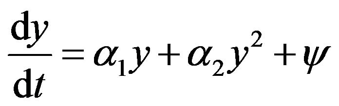 where
where  is normally distributed delta—correlated random value,
 .
.
The integration of the corresponding Fokker-Planck equation gives the steady-state solution in the form of bimodal distribution with unstable zero point, which is characteristic for many of the physical models—from spontaneous breakdown of symmetry in quantum physics to trigger modes in social and biological systems.
REFERENCES
- T. Bollerslev, “Generalized Autoregressive Conditional Heteroskedasticity,” Journal of Econometrics, Vol. 31, No. 3, 1986, pp. 307-327
- D. B. Nelson, “Conditional Heteroscedasticity in Asset Returns,” Econometrica, Vol. 59, No. 2, 1991, pp. 347- 370.
- R. Engle, “Estimating Time Varying Risk Premia in the Term Structure: The ARCH-M Model,” Econometrica, Vol. 55. No. 2, 1987, pp. 391-407.
- R. F. Engle and A. J. Patton, “What Good Is Volatility Model?” Quantitative Finance, Vol. 1, No. 2, 2001, pp. 237-245. doi:10.1088/1469-7688/1/2/305
- A. M. Avdeenko, “Chaos Structures. Multicurrency Adviser on the Basis of NSW Model and Social-Financial Nets,” 2011.
- A. M. Avdeenko “Multicurrency Adviser Based on the NSW Model. Detailed Description and Perspectives,” 2011.
- А. М. Авдеенко, “Стохастический анализ сложных динамических систем. Рынок Forex,” Нелинейный мир, 2010.
- H. Haken, “Information and Self-Organization,” Springer-Verlag, Berlin, Heidelberg, New York, 2000, 241 p.