Journal of Mathematical Finance
Vol.3 No.1A(2013), Article ID:29338,11 pages DOI:10.4236/jmf.2013.31A017
Price Forecasting and Analysis of Exchange Traded Fund
1College of Business, San Francisco State University, San Francisco, USA
2Department of Operations Management and Information Technology, HEC School of Management, Paris, France
Email: rameshb@sfsu.edu, igorsavin@gmail.com, kerbache@hec.fr
Received December 13, 2012; revised January 19, 2013; accepted January 24, 2013
Keywords: Forecasting; Pricing; ETF; Exchange Traded Fund; SPY; Holt’s Exponential Smoothing; Linear Regression; Multiple Regression; ARIMA Models
ABSTRACT
ETFs are baskets of securities designed to track the performance of an index. They are designed to provide exposure to broad-based indexes at a lower cost. We first analyzed why ETF should be the choice for an investment. We provide a brief history of this segment, key attributes of ETFs, and investments strategies and implementations with ETFs. The article then presents data analysis and a series of forecasting methods with data analysis techniques to evaluate the performance of each method. The data analysis and the forecast evaluation is to determine the best forecasting model for a single ETF (SPY). The different techniques considered include single exponential smoothing, Holt’s exponential smoothing, simple linear regression, multiple regression and various versions of Box-Jenkins (ARIMA) models. Based on the evaluation of a decade of past historical data, we provide a guidance for the price of our ETF (SPY) using the multiple regression technique (with an R-square of 98.4%), which produced promising results (with low forecast errors of 1% across several forecast metrics), among the different techniques evaluated. Promising results were also obtained using the Multiple regression technique on several other popularly traded ETF’s.
1. Introduction
Nearly everyone with some familiarity with US financial markets has heard the term Exchange Traded Fund (ETF) (Refer to [1-3] for more details.) The first of these products, the S&P 500 Depositary Receipts (SPDR, symbol SPY), which was launched in 1993 by the American Stock Exchange, allowed an investor to buy or sell the entire S&P 500 index within a single security. As the trading volume of the SPDR expanded, it served as a template for a host of products that replicated individual indexes and more recently, specific sectors and styles in the financial markets. Today, the NASDAQ 100-linked QQQQs are the most heavily traded symbols on any exchange, boasting average daily trading volume in excess of 100 million shares, representing almost $2.5 billion at current prices. The growth in trading volume of the more mature ETFs has spurred acceleration, particularly in the past three years, in the breadth of product offerings as institutional asset managers and exchanges have moved to capitalize on the popularity of these trading and investment vehicles. As of the first quarter of 2004, 155 U.S. Exchange Traded Funds exist, collectively representing nearly $161 billion in assets. Worldwide there are 296 ETFs trading in 15 countries.
Very simply, ETFs are baskets of securities designed to track the performance of an index. They are designed to provide exposure to broad-based indexes at a lower cost. Rather than buying shares from a mutual fund company, these shares are bought and sold on an exchange. Because ETFs trade like stocks, they provide many advantages over mutual funds. These include intraday liquidity, lower expenses, and tax efficiency, as indexes are required to sell holdings only when index components change. You have lower risk due to diversification.
Unfortunately, owning one stock leaves you susceptible to analyst downgrades, disappointing earnings, accounting issues or an unperceived negative event. With an ETF, you will own an underlying basket of stocks giving you market exposure with less risk. ETFs are simpler to track than mutual funds because they disclose their holdings daily and differ from closed-end funds in that new shares can be created or redeemed on a daily basis by a market maker.
So, what is the need for ETF’s forecast? Fortunes are acquired and lost in the stock market. Today, we employ multiple tools to help us gauge the direction of the market using techniques ranging from fundamental and technical analysis to macro analysis. Included in the list, are the forecasting techniques that help us understand and forecast the direction of the market. It should never be used independently, but together with other models, it helps to determine the long term market direction.
Specifically, the objective of this research is to construct forecast for a single ETF, utilizing a time-series forecasting technique. This study includes data for symbol: SPY. The Standard and Poor’s Depositary Receipts (SPDRs) Trust seeks to correspond generally to the performance, before fees and expenses, of the S&P 500 Index. SPDR Trust is an exchange-traded fund that holds all of the S&P 500 Index stocks. The time period is from January 29, 1993 to March 28, 2005. A series of forecasting models were established and tested to find the most appropriate one.
The study is limited to date from January 29, 1993 to March 28, 2005 due to SPY only starting to trade in 1993. However, further development of S&P 500 historical data, which SPY mirrors, should help us incorporate a better informed decision on what technique to use. One important fact which is outside the scope of the paper is that the ETF price is subject to change due to certain set of economic factures which influence effectively projecting the future price.
We also discuss in a separate section the guidance of forecasts from March, 2005 to June, 2008 of our best forecasting technique (Multiple regression), and the excellent performance of our technique in comparison with the actual data during this period (forecast errors less than 2%).
2. A Brief Review of the Origins and History
In its application, Exchange Traded Funds evolved from the index mutual fund, first successfully brought to market in the mid-1970 by Vanguard Investments and its founder, John C. Bogle. The hugely successful Vanguard index funds were a natural choice as a model, and State Street was able to essentially match the 20 basis point annual fee that Vanguard charged for its S&P 500 fund. In late January 1993, the AMEX launched the S&P 500 Depositary Receipts (SPDR), and the ETF industry was born. The Spiders, as they became known, were an instant success. Average daily volume in the first full month of operation was over 300,000 shares per day, and within a few years, volume regularly hit over 1 million shares a day.
3. The Key ETF Attributes
During the first year of operation, the SPDR trust had less than $1 billion in assets. Since then, assets in the ETF industry have mushroomed roughly 100 fold, to nearly $161 billion, as illustrated in Figure 1. The most important drivers of their popularity are their combination of low costs, liquidity, and tax efficiency, delivered in the simple form of a single stock.
3.1. Costs
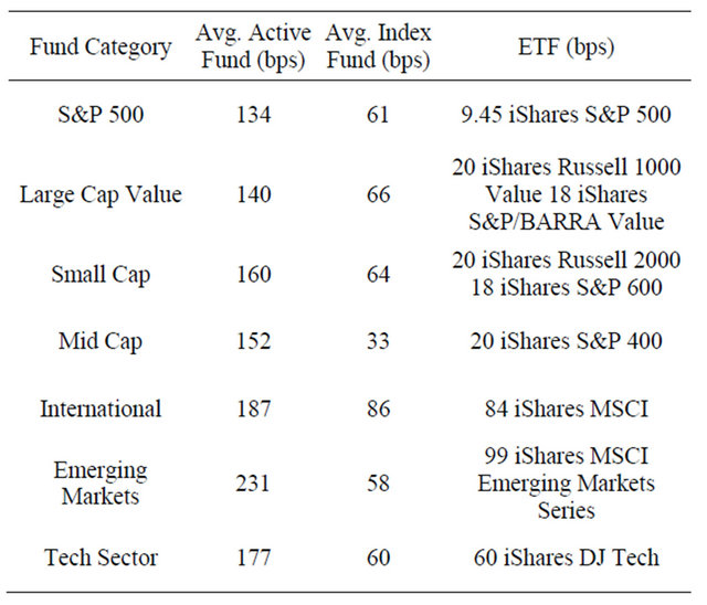
Annual management fees for ETFs range from 9 basis points for the iShares S&P 500 fund to 60 basis points for some domestic sector funds, to 99 basis points for some foreign country-specific funds. According to Lipper Analytical Services, the 9 basis point fee that iShares charges for its S&P 500 fund is less than half of the average expense ratio paid by investors in traditional mutual funds designed to track the same index. ETF expense ratios also compare favorably to the average 75 basis point annual fee incurred by investors in passive mutual funds. When compared to actively managed funds, however, the difference in cost becomes more significant. Exchange traded funds, like index mutual funds, lack the overhead in the form of extensive research and trading operations that active funds require. Additionally, the broker-dealer does all shareholder accounting where the securities are held. This eliminates the need for a transfer agent to track shareholders, a significant cost advantage versus traditional mutual funds. These cost-savings are then passed to the investors, as the following Tables 1 and 2 reveal.
3.2. Liquidity
Liquidity is another area of critical concern to investors, particularly to institutions. The two major determinants of liquidity in a security are the bid-offer spreads and the size or depth of the market. Despite their relative youth, the largest and best known ETFs provide liquidity that rivals the top-tier large cap stocks such as IBM, WalMart, and GE. The QQQQ, currently the most actively
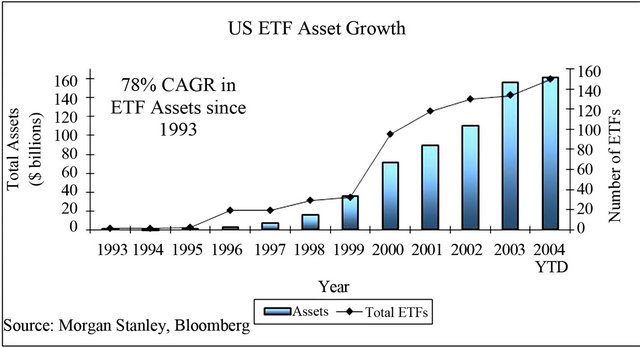
Figure 1. US ETF Asset Growth.
Table 1. Annual expense ratios (in basis points).
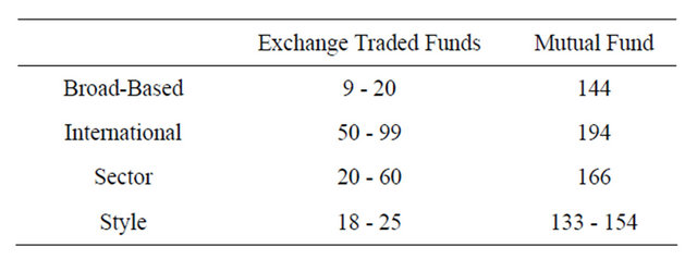
Table 2. Fund Category and the corresponding ETFs.
traded stock on any exchange, trades over 100 million shares in daily volume, typically with a bid-ask spread of roughly 4 cents, or 0.15% at current prices. Institutional trading desks routinely handle 100,000 share blocks of the QQQQs and the Spiders on a daily basis, demonstrating the depth of the markets for these funds. Shortly after the SEC announced in early July 2004 that corporate executives would have to swear to their financial results, spider trading averaged almost 60 million contracts a day—nearly triple the average volume for the year. Of course, the liquidity of an individual fund is ultimately tied to the liquidity of the underlying stocks. Some of the more recent additions to the ETF universe have yet to develop anywhere near the level of liquidity provided by the broad market funds. As interest in the sector continues to grow, liquidity will likely come to many of the newer entrants, while the fund providers will dissolve those that do not gain traction.
3.3. Tax Efficiency
Tax efficiency is a particular strength of Exchange Traded Funds, for two reasons. First, like index mutual funds, portfolio turnover is kept to the absolute minimum, as positions change only as the index constituent change, typically on an annual basis. This low turnover minimizes the number of taxable events realized in the fund, resulting in low realized capital gains being passed to investors at the end of each year. Figure 2 shows how portfolio turnover with equity funds has increased over time.
Second, the structure of ETFs allows them to outperform even index funds with respect to minimizing the tax burden borne by investors. Typically, when an index fund receives redemptions from an investor, the fund must sell some portion of its holdings to generate the cash to meet that redemption. (By design, index mutual funds never carry cash, which would distort the funds ability to mirror the performance of the index.) The sale of the fund’s holdings to meet the redemption represents a taxable event that is then passed along to all of the fund shareholders in the form of a realized capital gain. Almost all ETFs avoid this problem through a mechanism known as redemption in kind or payment in kind. What are known, as qualified participants—the institutions that trade in large blocks of ETF shares—are able to redeem ETF shares for shares in the underlying securities. No cash changes hands, as is the case with a mutual fund, and no taxable event takes place for the ETF. (The creation and redemption process will be discussed in more detail later.) As Table 3 illustrates, taxes take a significant bite out of a mutual fund investors’ return.
3.4. Transparency
Any investor wishing to know the exact constituents of a particular ETF can go to the sponsoring company’s website and quickly obtain that information, updated on a daily basis, complete with the weightings of the individual stocks in the fund. In contrast to this transparency of
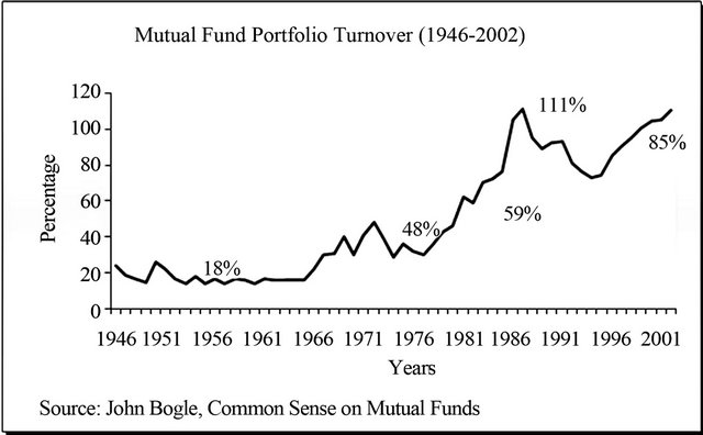
Figure 2. Mutual fund portfolio turnover.
Table 3. Pre-tax versus after-tax returns.
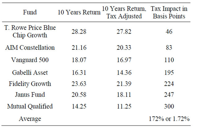
Source: David Lerman, Exchange Traded Funds and E-Mini Stock Index Futures.
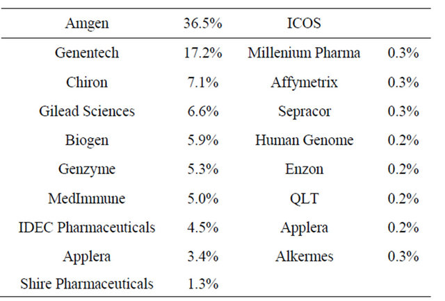
ETFs’, the typical mutual fund discloses it holdings on a quarterly or semi-annual basis. Often, information regarding the top ten holdings in a particular mutual fund is available on a more regular basis, but that degree of transparency cannot be compared to that of ETFs’. With the transparency inherent to ETFs, the investor can protect himself from what has become known in the mutual fund industry as “style drift”. Frequently, a mutual fund manager charged with a particular style of investing will, for a variety of reasons, stray to varying degrees from their initial charter. Although generally done in search of perceived higher returns, style drift can distort the performance characteristics of a managed portfolio to the detriment of the fund holder. The below tables (Tables 4 and 5) provide two examples of the composition of an ETF.
3.5. Intra-Day Trading Access
Buy and hold indexers like John Bogle would surely cringe at the notion of day-trading the market. Flipping
Table 4. iShares Russell 2000 Index (IWM)—consists of 1907 stocks with a breakdown as follow.
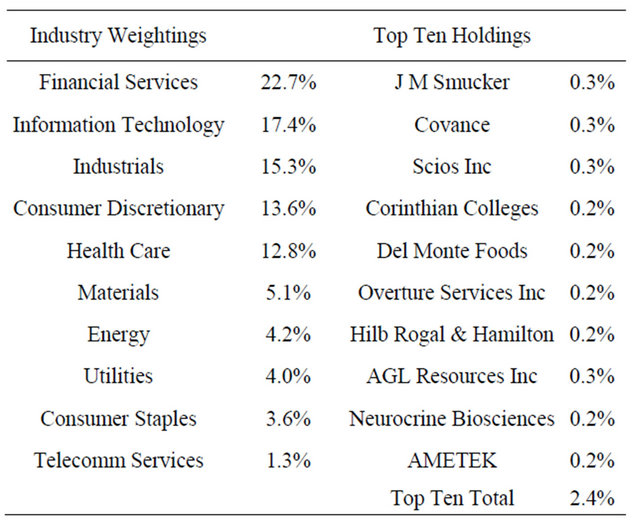
Table 5. Biotech HOLDRS (BBH)—consists of 19 stocks.
the Spiders throughout the day, paying a brokerage commission each time, tends to defeat the purpose of indexing, whose primary goal is to reduce costs and allow market gains to compound over time. However, the ability to buy and sell ETFs throughout the trading day has unquestionably enhanced the popularity of Exchange Traded Funds, and in so doing, increased trading volumes and liquidity. As such, this intra-day liquidity stands as a significant evolution of the index mutual funds that preceded the ETF. ETFs trade just like stocks throughout the day, as well as after-hours on the electronic exchanges such as Instinet. Some of the broad market linked funds, such as those linked to the Russell indexes, the S&P 500, and the Dow Jones Industrial Average actually trade until 4:15 PM (EST), fifteen minutes longer than individual stocks trade. Brokerage commissions for Exchange Traded Funds also typically mirror those of stocks listed on the major exchanges.
3.6. No Uptick Rule on Short Sales
Unlike individual stocks, Exchange Traded Funds require no uptick in the share price to make a short sale. This allows speculators and institutional hedgers playing ETF markets to obtain short exposure as easily as they can go long. While shorting an index is antithetical to the indexers who paved the way for ETFs, the no uptick rule has helped drive ETF trading volumes up, with an attendant increase in liquidity for all participants.
4. ETF Players
The fund managers and their primary custodians are Barclays Global Investors (iShares), the Bank of New York (Index Trusts), Merrill Lynch and the Bank of New York (HOLDRS), Vanguard (VIPERS), and State Street Global Advisors (SPDRs and street TRACKS). Figure 3 below shows the total assets invested in U.S. in the ETF universe.
5. Strategies and Implementations
With several strategies to choose from, you have many
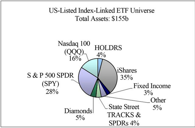
Figure 3. US-listed index-linked ETF universe.
options when investing in ETFs. Asset allocation, hedging, sector bets, index replication, cash equalization, gaining international exposure and tax strategies are all examples.
5.1. Asset Allocation
The simplest is to use ETFs for asset allocation. Until recently, asset allocation was difficult for individual investors due to costs and assets required to attain the correct levels of diversification. With their low cost and ease of use, ETFs are an easy way to gain market exposure to many broad-based indexes or style indexes in one single security. Because they cover a broad range of style and size spectrums, as well as sector-specific funds, investors can build a customized portfolio consistent with their risk tolerance and investment horizon. The DJ Industrial Average (DIA), iShares Russell 1000 (IWB) and Vanguard Total Stock Market VIPERs (VTI) are all examples of this. Figure 4 illustrates a typical asset allocation matrix.
5.2. Hedging
Another strategy is hedging. Given their structure, making hedges and sector bets are easy with ETFs. If you have a negative view of the market, you can sell short ETFs. Since there is no downtick rule, ETFs are even easier to trade than a stock. If you have a negative bias toward the market near term, you can sell short some of the broader market ETFs mentioned above. If you are right, this would offset losses in your portfolio should the market decline.
5.3. Sector Bets
There are 24 US-listed ETFs representing US market sectors and 25 industry-specific ETFs. With all of the sector ETFs and HOLDRS instruments to choose from, participation in almost any industry is possible. If you
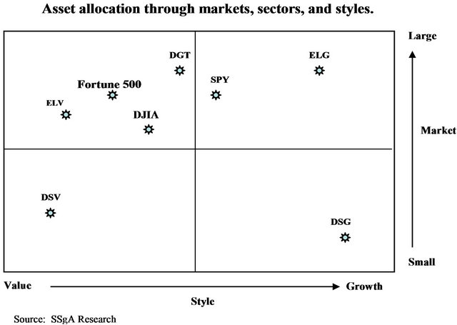
Figure 4. Asset allocation through markets, sectors, and styles.
feel the telecomm industry is going to recover but question which companies to buy first, the Telecom HOLDRS (TTH) would be a likely purchase. If you are looking for a basket of defensive names, the composition of iShares DJ US Real Estate Index Fund (IYR), Energy Select Sector SPDR Fund (XLE) and the iShares DJ US Utilities Sector Index Fund (IDU) are examples of what you may buy. If you are certain the Internet is going to make a comeback, you could look at the Internet HOLDRS (HHH) or Internet Infrastructure HOLDRS (IIH). With so many individual sector funds available, this provides extreme flexibility.
5.4. Index Replication
An investor seeking broad-market exposure can create returns that resemble a major index by buying a basket of sector ETFs. By acquiring individual sector ETFs in the correct amounts, an investor can replicate a major index such as the S&P 500 or the Dow Jones Index. In a similar manner, a basket of nine sector SPDRs could create an overall portfolio similar to the S&P 500 Index. Owning sector funds in the proper proportion can produce a similar return to the Dow Jones US Total Market Index, with the added advantage of having the capability to realize gains or losses in the individual sectors. This would not be possible if only a single index fund was purchased. Figure 5 shows an example of index replication.
5.5. Cash Equalization
Cash equalization is a strategy that helps mitigate what is known as cash drag. Portfolio managers are not paid to hold cash. At times when there is a considerable amount of cash coming in the door, managers may have a hard time keeping up. If a fund holds even small amounts of cash while the market is going up, it would under perform its benchmark. By purchasing ETFs, investors can gain quick exposure until they decide what to add to their portfolio. The same can be said for individual investors who have not done enough research to make an informed investment decision.
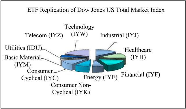
Figure 5. ETF replication of Dow Jones US total market index.
5.6. International Exposure
Investing overseas has been the topic of much debate. Some feel it is an easy way to take advantage of opportunities that have already been exploited in mature markets in the US. Others feel it provides no diversification. If you look at the severe declines over the past 18 years in the US, equally severe drops in international markets have followed them. However, billions of US dollars reside in international stocks and funds. ETFs offer a way to gain broad exposure across many overseas markets as well as individual countries through the MSCI iShares series. Given the current state of affairs in the US; fighting a war, the weakening dollar and an economy that needs a jumpstart, looking overseas would have been a smart idea. The iShares MSCI South Korea Index Fund (EWY) is up 26.6% from a year ago while the iShares MSCI Austria Index Fund (EWO) is up 20% since its inception last November.
5.7. Tax Strategies
ETFs are useful in tax planning strategies and help avoid the IRS wash sale rule. For example, say you have gains due to the healthcare exposure in your portfolio but losses in your energy stocks. You could offset your gains by selling the underperforming stocks, your energy names. If you feel the energy sector is going to recover and want to have exposure, yet do not want to be victim to the wash sale rule by buying back those names, you can purchase the Energy Select SPDR (XLE). By purchasing a completely different security, you still have your energy exposure and will not be affected by the wash sale rule.
ETFs have experienced extraordinary success to date. Some market estimates are predicting asset growth between $300 billion and $500 billion by end of 2007. Given the growth ETFs have experienced since their inception, these figures are not out of the question. The media has targeted ETFs mainly as investments for the average retail investor. The reality is ETF activity is highest among institutions. Critics say ETFs may follow in the footsteps of traditional mutual funds and grow in number well over 8000.
6. Research Design
This research utilizes time series forecasting method because of the plausible pattern already pre-existing in the historical data. Furthermore, short-term forecasting tends to use the recent stock price to reflect the continuous change in the stock market.
For this project, Minitab’s time series functions in the statistics menu are mainly used to complete the forecasting research. Four measures of accuracy are used: Average Error, Mean Squared Deviation (MSD), Mean Absolute Deviation (MAD) and Mean Absolute Percentage Error (MAPE).
7. Data Analysis and Testing
The financial section at http://finance.yahoo.com provides up to date information on majority of the publicly traded symbols in the US and World Market. It further provides historical data going back to 1993 for majority of the symbols traded.
For this research and other of similar scope, symbol price is plotted against time. It is followed by decomposition of patterns (trend, cyclical, seasonal, and irregular). This will give us an overview of how each component contributed to the stock price and a better understanding of what forecasting technique to use. The adjusted stock price, adjusted for dividends and splits, is plotted against time in Figure 6 (monthly data) to provide an illustration of the data.
As one can see there is a clear trend in this graph. We also suspect the presence of a cyclical component as well, due to business cycles. Although a number of different techniques can be used, we use the ones that are most effective for our data characteristics. The forecasting methods we experimented include: Price Differences, Single/Holt’s Exponential Smoothing, Simple Linear Regression, Multiple Regression and several versions of Box-Jenkins (ARIMA) models (refer to [4-10] for discussion on these techniques).
After selecting the forecasting methods, the monthly price data is used to estimate the parameters for each model, and the forecast accuracy of the technique was calculated. This research was conducted in 2005, and we had a total of 148 data points over 12 years (Jan 1993 through March 2005). We used the first 124 data points (Jan 1993 through March 2003) as our base to construct the forecast equation for the selected forecasting techniques and the accuracy is tested over the remaining 24 data points (March 2003 through March 2005). Note that, the actual data is available for these 24 data points
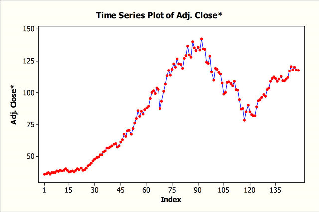
Figure 6. Time series plot of adjusted stock price.
(March 2003 through March 2005), and the forecast for these data points is based on our experimented forecasting techniques.
Later, in a separate section, we also provide guidance on forecasts from March, 2005 to June, 2008 and its forecast accuracy, using the best forecasting technique.
7.1. Differences of Prices
Figure 7 show the fit for this technique.
7.2. Single Exponential Smoothing
Figure 8 shows the fit for this technique.
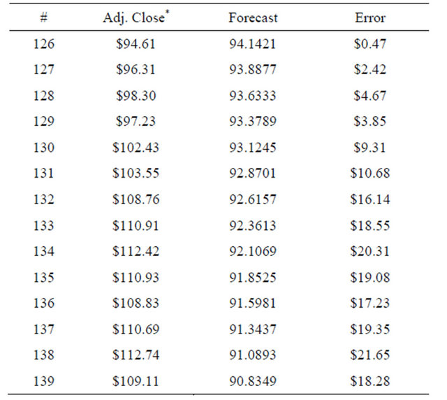
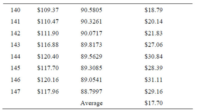
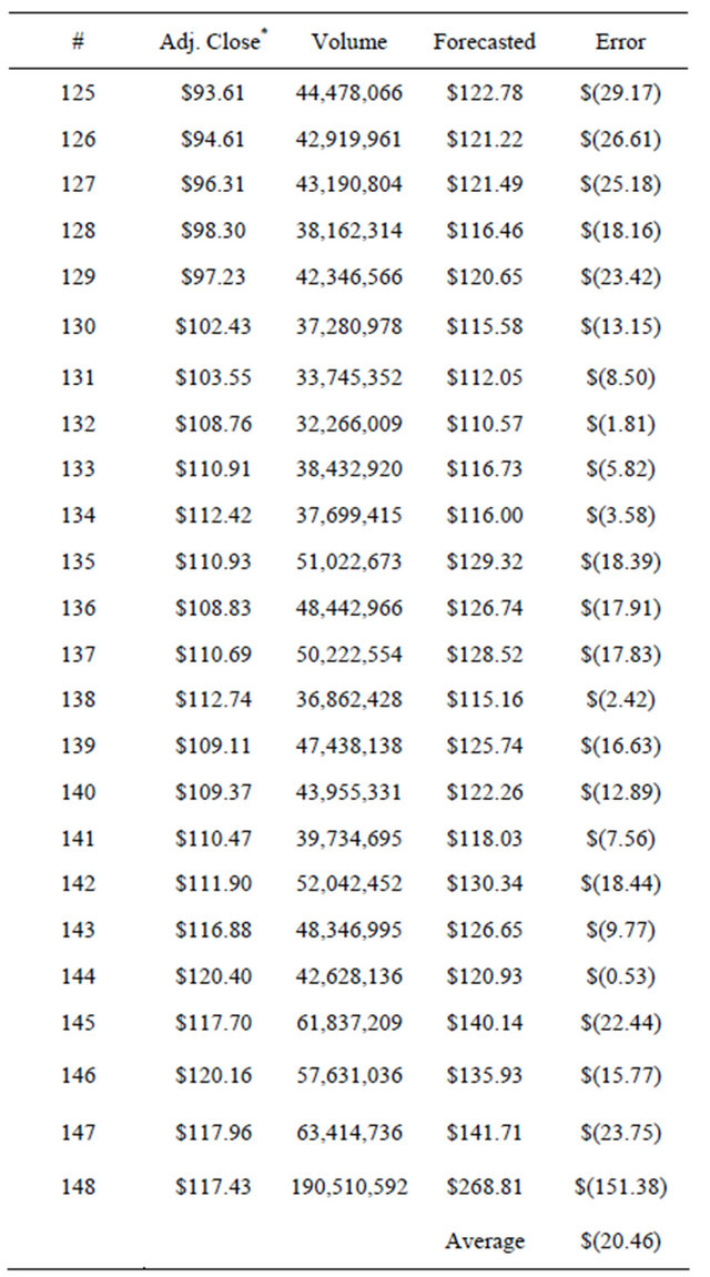
Tables 6 and 7 show the forecast for data points 125 through 148 (Jan 1993 through March 2005) using Simple Exponential Smoothing and Holt’s Exponential Smoothing respectively.
7.3. Holt’s Exponential Smoothing
Figure 9 shows the fit for Holt’s Exponential Smoothing technique.
7.4. Simple Linear Regression
The regression equation obtained from MINITAB is Adj. Close* = 78.3 + 0.000001 VolumePredictor Coef SE Coef T P Constant 78.344 2.994 26.16 0.000 Volume 0.00000052 0.00000011 4.930.000
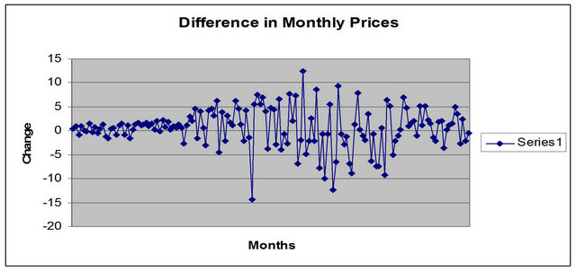
Figure 7. Difference in monthly prices.
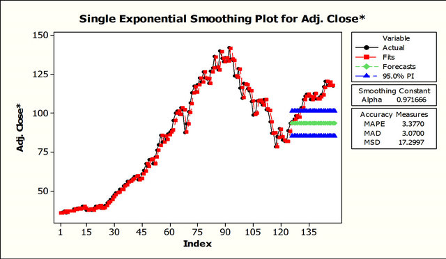
Figure 8. Single exponential smoothing for adjusted stock price.
Table 6. Forecast for data points 125 through 148 using Simple Exponential Smoothing.
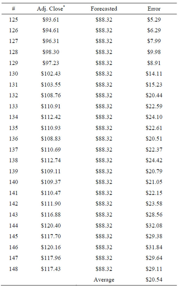
Table 7. Forecast for data points 125 through 148 using Holt’s Exponential Smoothing.
Continued
MAPE: 3.3770; MAD: 3.0700; MSD: 17.2997.
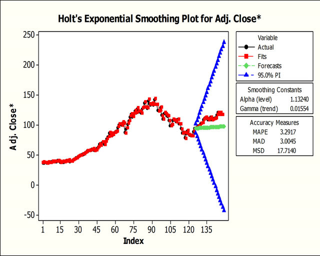
Figure 9. Holt’s exponential smoothing for adjusted stock price.
S = 29.9692 R-Sq = 14.3% R-Sq(adj) = 13.7% Analysis of Variance Source DF SS MS F P Regression 1 21849 21849 24.33 0.000 Residual Error 146 131131 898 Total 147 152979 S = SQRT(MSE), MSE = S 2 = 29.96922 = 856.6685 Tables 8 below show the forecast for data points 125 through 148 (Jan 1993 through March 2005) using Linear Regression method.
Here, we can see that simple volume is not a very good predictor of the stock price. However, we commonly use known variable transformations (including log(x), 1/x, square root of X and, X square) to determine which correlates better.
Log(x)
S = 19.6300 R-Sq = 63.2% R-Sq(adj) = 63.0% SQRT (X)
S = 25.9292 R-Sq = 35.9% R-Sq(adj) = 35.4% X*X S = 31.1564 R-Sq = 7.4% R-Sq(adj) = 6.8% 1/X S = 21.9129 R-Sq = 54.2% R-Sq(adj) = 53.9% As we can observe, a simple variable transformation from volume to Log(volume) significantly improves the Linear regression technique. However, this still is inadequate for our purposes and we need to add more variables into the mix.
7.5. Multiple Regression
We review the following data available to us to determine the independent variables in our Multiple regression study (refer to [11,12]): date, open price, high price during the day, low price during the day, close of the day, volume of shares traded, adjusted close price (adjusted for dividend and splits). It is not unreasonable to assume
Table 8. Forecast for data points 125 through 148 using Linear Regression method.
MSE: 856.6685; MAD: 5.13; MAPE: 5.07.
that more than only one variable contributes to the adjusted close. However, we saw that volume doesn’t explain the adjusted close. We can’t use open price, high price, or low price because they are derived from the close dates during the period. Our only other straight forward option is to use date as another predictor. However, this might work theoretically, but doesn’t really make sense. We need to come up with our own predictor derived from data given to us. Below are the statistical results when using different averages of previous closes:
6 Months:
S = 6.38050 R-Sq = 95.9% R-Sq(adj) = 95.8% 5 Months:
S = 5.93360 R-Sq = 96.5% R-Sq(adj) = 96.4% 4 Months:
S = 5.49330 R-Sq = 97.0% R-Sq(adj) = 97.0% 3 Months:
S = 4.99514 R-Sq = 97.5% R-Sq(adj) = 97.5% 2 Months:
S = 4.57251 R-Sq = 98.0% R-Sq(adj) = 97.9% 1 Months (use last months value as a predictor):
S = 3.29720 R-Sq = 99.0% R-Sq(adj) = 98.9% We observe that using last month’s value is the best predictor of this month’s value with an average variance of $0.56 we use the following predictors for our multiple regressions: last month’s adjusted close and volume.
The regression equation is Adj. Close* = 0.28 + 0.980 Average + 0.129 LOG (volume)
Predictor Coef SE Coef T P Constant 0.284 3.582 0.08 0.937 Average 0.98027 0.01796 54.59 0.000 LOG(volume) 0.1295 0.3060 0.42 0.673 S = 4.16821 R-Sq = 98.3% R-Sq(adj) = 98.3% Analysis of Variance Source DF SS MS F P Regression 2 146949 73475 4229.00 0.000 Residual Error 143 2484 17
Total 145 149434 S = SQRT(MSE), MSE = S2 = 4.168212 = 17.3739746 Refer to Table 9 for a detail forecast. As we can see, our R-square is 98.4% with S being 4.156.
When we do a fitted line plot, using the quadratic model, we even increase our R-Sq and S slightly (see Figure 10).
Figure 11 illustrates our forecasts using different methods for the previous twelve 12 months when compared to the actual adjusted close.
7.6. Box-Jenkins (ARIMA) Models
Through the plot of the data for the first 124 data points, the next step was to identify a tentative model to look at the sample autocorrelations of the data. We observed that the first several autocorrelations are persistently large and trailed off to zero rather slowly. We then differenced the data to eliminate the trend and create a stationary series. A plot of the differenced data appeared to vary about a fixed level.
The sample autocorrelations and the sample partial autocorrelations for the differences are then plotted. Comparing the autocorrelations with their error limits, the only significant autocorrelation was at lag 1. Similarly, only the lag 1 partial autocorrelation was significant. The autocorrelations appear to cut off after lag 1, indicating MA (1) behavior. At the same time, the partial autocorrelations appear to cut off after lag 1, indicating AR (1) behavior. Neither pattern appears to die out in a declining manner at low lags. So, we decided to fit both ARIMA (1,1,0) and ARIMA (0,1,1) models to our data (refer to [13])
ARIMA (1,1,0) model for Adj Close
Final Estimates of Parameters
Table 9. Forecast for data points 125 through 148 using Multiple Regression method.
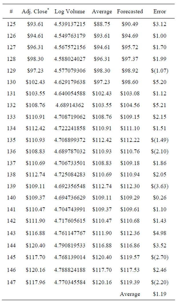
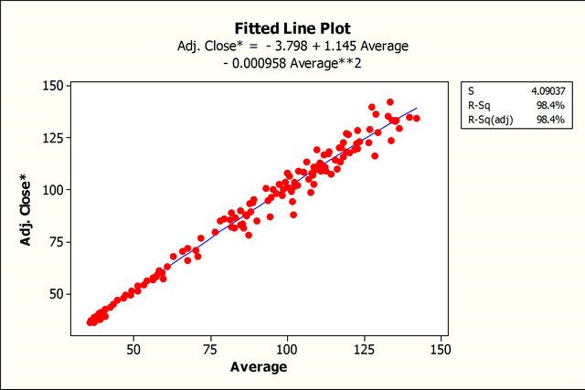
Figure 10. Fitted line plot for adjusted stock price.
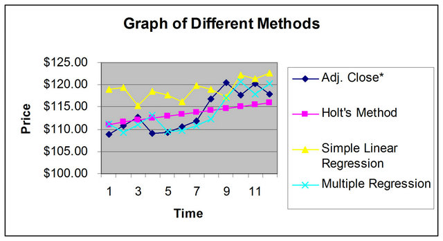
Figure 11. Forecasts using different methods.
Type Coef StDev T P AR 1 −0.0483 0.0901 −0.54 0.592 Constant 0.4697 0.3737 1.26 0.211 Differencing: 1 regular difference Number of observations: Original series 126, after differencing 125 Residuals: SS = 2147.19 (backforecasts excluded)
MS = 17.46 DF = 123 Modified Box-Pierce
(Ljung-Box) Chi-Square statistic Lag 12 24 36 48 Chi-Square 9.8 18.6 27.3 45.6 DF 10 22 34 46 P-Value 0.462 0.667 0.785 0.490
ARIMA (0,1,1) model for Adj Close
Final Estimates of Parameters Type Coef StDev T P MA 1 0.0563 0.0900 0.63 0.533 Constant 0.4478 0.3526 1.27 0.206 Differencing: 1 regular difference Number of observations: Original series 126, after differencing 125 Residuals:
SS = 2146.32 (backforecasts excluded)
MS = 17.45 DF = 123 Modified Box-Pierce
(Ljung-Box) Chi-Square statistic Lag 12 24 36 48 Chi-Square 9.8 18.8 27.5 45.8 DF 10 22 34 46 P-Value 0.458 0.659 0.779 0.482 We then computed the Average error, MAD, MSE, MAPE for these two ARIMA models. The results are as follows;
ARIMA (1,1,0): Average Error: 8.56, MAD: 8.59, MSE: 94.80, MAPE: 8.04 ARIMA (1,1,0): Average Error: 8.58, MAD: 8.62, MSE: 95.16, MAPE: 8.06 As we can notice, both models result in similar performance, and is consistent with our evaluation of the autocorrelation and partial autocorrelations of the differenced data.
Finally, note that, Multiple regression models performed the best among all the forecasting techniques tested.
7.7. Guidance based on Multiple Regression from March 2005 through June 2008
Our study was conducted in year 2005 and hence recently we used our best forecasting technique to gauge how well we performed over the last 3 years using the forecasts computed with Multiple Regression. We now know the actual demand for the data points 148 through 186 (i.e. March 2005 through June 2008). Based on testing over these data points, we computed the Average error, MAD, MSE, MAPE over these 39 month period.
Average Error: 2.01, MAD: 3.036, MSE: 13.21, MAPE: 2.48.
We thus confirm the excellent performance of our Multiple Regression model.
We present in Table 10 the most popular ETFs by volume.
We used our analysis on the second most traded ETF today, SPDR. Now, we will use our best forecasting technique, multiple regressions, and apply it to the rest of the top 4 most traded ETFs: NASDAQ 100 Trust Shares, Semiconductor HOLDRs, Energy Select Sector SPDR, and iShares Russell 2000 Index. It is important to note that some of them do not have the historical basis like the SPDR; for example NASDAQ 100 Trust Shares only goes back to 1999.
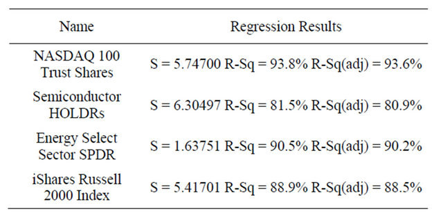
Regression Results are shown in Table 11.
As we can see, the technique works better on more diversified group like the NASDAQ 100 but at the same time, the rest have a significant correlations to our inputs as well. As one can tell, prior to investing in these ETFs, one needs to do other research including fundamentals of underline companies, macro of economy and sectors, but our forecasting technique (Multiple regression) provides a good initial guidance.
Table 10. Most Popular ETFs by volume.
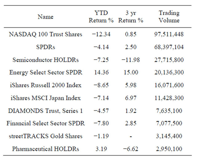
Table 11. Regression Results.
8. Summary and Conclusions
Currently, raw data is available in great amounts on the stock market. This unprecedented turn of events has democratized the stock market in one way or another. Everyone, not only the large financial corporations, has access to the data for free or low cost and everyone can build their own individual models. Using the methods that we outlined, a person can get a quick grasp at the direction of the market and can make a more informed decision than before.
In this paper, we presented and compared several forecasting techniques to provide guidance for the price of our ETF (SPY). The underlying concept was that this is only one of the tools to predict the price of the ETF. The analyst needs to do technical and fundamental analysis, develop macro models, and talk to management in companies, to successfully trade in the market. However, our forecasting techniques provide a good initial guidance that could be used in assessing any given ETF in the trading market, as shown on four other popularly traded ETFs.
The different techniques considered include Single exponential smoothing, Holt’s exponential smoothing, Simple linear regression, Multiple regression and BoxJenkins models. Based on the evaluation of a decade of past historical data, we provide future guidance for the price of our EFT (SPY) using the Multiple regression technique (with an R-square of 98.4%), which produced promising results (with forecast errors of 1% across several forecast metrics), among the different techniques evaluated. Promising results were obtained using Multiple regression on several other popularly traded ETF’s.
9. Acknowledgements
The first author, Ramesh Bollapragada would like to thank the college of business, San Francisco State University and HEC School of Management, Paris for providing a conductive atmosphere to conduct this research. Further, he would like to dedicate his contributions to his parents, Rajarao Bollapragada and Mangatayaru Dulla Bollapragada, who were a great source of inspiration in his entire academic career.
REFERENCES
- http://www.google.com
- http://finance.yahoo.com
- http://www.morningstar.com
- J. S. Armstrong, “Principles of Forecasting: A Handbook for Researchers and Practitioners,” Kluwer Academic Publishers, Norwell, 2001.
- G. E. P. Box, G. M. Jenkins and G. C. Reinsel, “Time Series Analysis: Forecasting and Control,” Third Edition, Upper Saddle River, Prentice Hall, 1994.
- S. Chopra and P. Meindl, “Supply Chain Management, Strategy, Planning & Operation,” Third Edition, Upper Saddle River, Prentice Hall, 2007.
- F. X. Diebold, “Elements of Forecasting,” Third Edition, Cincinnati, South-Western, 2004.
- J. E. Hanke and D. W. Wichern, “Business Forecasting,” Eightth Edition, Upper Saddle River, Prentice Hall, 2005.
- S. Makridakis, S. C. Wheelwright and R. J. Hyndman, “Forecasting Methods and Applications,” Third Edition, John Wiley & Sons, New York, 1998.
- P. Newbold and T. Bos, “Introductory Business and Economic Forecasting,” Second Edition, Cincinnati, SouthWestern, 1994.
- T. Dielman, “Applied Regression Analysis for Business and Economics,” Third Edition, Pacific Grove, Duxbury, 2001.
- J. Yurkiewicz, “Forecasting 2000,” OR/MS Today, 2000, pp. 58-65.
- D. J. Pack, “In Defense of ARIMA Modeling,” International Journal of Forecasting, Vol. 6, No. 2, 1990, pp. 211-218. doi:10.1016/0169-2070(90)90006-W