ABSTRACT

In this paper we study a multivariate extension of a structural credit risk model, the CreditGrades model, under the assumption of stochastic volatility and correlation between the assets of the companies. The covariance of the assets follows two popular models which are non-overlapping extensions of the CIR model to dimensions greater than one, the Wishart process and the Principal component process. Under CreditGrades, we find quasi closed-form solutions for equity options, marginal probabilities of defaults, and some other major financial derivatives.

1. Introduction

We present a structural credit risk model which considers stochastic correlation between the assets of the companies. We allow the covariance of the assets to follow two popular stochastic covariance models. First we assume it follows a Wishart process [1] then we assume a Principal component Process (see [2]), both are non overlapping extensions of the CIR model to dimensions greater than one.

Modeling stochastic correlation has difficulties from the analytical as well as the estimation point of view. One of the attempts to x this gap began with a paper on Wishart processes by [1], which followed by a series of papers by Gourieroux, see [3]. Several authors have recently brought the finance community’s attention to the Wishart process and showed that the Wishart process is a good candidate for modeling the covariance of assets. A Wishart process is an affine symmetric positive definite process. The stream of papers [3-7] brought the finance community’s attention to this process as a natural extension of Heston’s stochastic volatility model, which has been a very successful univariate model for option pricing and reconstruction of volatility smiles and skews. The popularity of the Heston model as well as the empirical evidence of stochastic correlation and volatility has contributed to the recent popularity of the Wishart process. Risk is usually measured by the covariance matrix. Therefore Wishart process can be seen as a tool to model dynamic behavior of multivariate risk. Via the Laplace transform and the distribution of the Wishart process [3], prices derivatives with a generalized Wishart stochastic covariance matrix. This approach can be used to model risk in the structural credit risk framework. DaFonseca extends his approach in [7] to model the multivariate risk by a Wishart process. In this paper several risky stocks are considered and the pricing problem for one dimensional vanilla options and multidimensional geometric basket options on the stocks is presented. We adapt existing results about the Wishart process to the structural CreditGrades framework. We give quasi closed-form solutions for equity options, marginal probabilities of defaults, and some other major financial derivatives. For calculation of our pricing formulas we make a bridge between two recent trends in pricing theory; from one side, pricing of barrier options by [8] and [9] and from other side the development of Wishart process by [1].

In the second part of the paper we develop a new model for credit risk based on a model with stochastic eigenvalues called principal component stochastic covariance. To induce the stochasticity into the structure of volatilities and correlation, we assume that the eigenvectors of the covariance matrix are constant but the eigenvalues are driven by independent Cox-Ingersoll-Ross processes. To price equity options on this framework we first transform the calculations from the pricing domain to the frequency domain. Then we derive a closed formula for the Fourier transform of the Green’s function of the pricing PDE. Finally we use the method of images to find the price of the equity options. Same method is used to find closed formulas for marginal probabilities of defaults and CDS prices. Inspired by the standard stochastic volatility models starting from Heston’s paper [10] and the work on [2] the applications of the principal component model in credit risk is studied. The main idea is to identify the covariance matrix by its eigenvectors and eigenvalues. In the above papers, authors have assumed that the eigenvector of the covariance matrix are constant but the eigenvalues follow a CIR process. This implies a stochastic structure for the correlation between the assets. [2] prices the collateralized debt obligations under the Merton’s model using a tree approach and the principal component model.

Merton’s model [11] is the first structural credit risk model proposed which considers the company’s equity as an option on the firm’s asset. There has been numerous extensions for the Merton’s model in the literature including incorporating early defaults, stochastic interest rates, stochastic default barriers and jumps in the asset’s price process. A simpler approach was jointly developed by CreditMetrics, JP Morgan, Goldman Sachs and Deutsche Bank, called the CreditGrades model, this can be seen as a particular case of Merton with zero time to maturity. The simplicity allows for closed for expression on some derivatives as shown in our paper which can not be found closed form under Merton or Black Cox structural frameworks. We extend the CreditGrades model using stochastic covariance Wishart process focusing on the role of stochastic correlation. The performance of a company is usually monitored by observing its equity’s volatility or the CDS spread. CreditGrades model can be considered as a down-and-out barrier credit risk model. This means that default is triggered if the value of the asset reaches a certain level identified by the recovery part of the debt. [12] has extended the CreditGrades model to price equity options by introducing the equity as a shifted log-normal process. [9] has extended [12] idea by embedding the Heston’s volatility into the model and pricing equity derivative. Both [9] and [12] models are univariate credit risk models. We extend the CreditGrades model by use of the Wishart and PC processes to dimensions greater than one implementing stochastic correlation into the dynamics of the assets. We give quasi closed formulas for equity derivatives based on these models.

This paper is organized as follows: in section 2 we use Wishart process as a candidate to model the covariance matrix of the assets’ prices within a CreditGrades model. The pricing problem for some derivatives on the equities is derived in section 2.2. Section 3 presents and uses the Principal component process for the covariance matrix of the assets’ prices within the same structural framework. The pricing problem is derived in Section 3.2. Section 4 concludes. The proofs are given in the appendix.

2. The CreditGrades Wishart Process

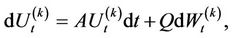
In this section, we introduce our Wishart CreditGrades model. CreditGrades model is a version of the Merton model jointly developed by CreditMetrics, JP Morgan, Goldman Sachs and Deutsche Bank. The original version of the CreditGrades model assumes that volatility is deterministic. We extend CreditGrades model, by means of stochastic covariance Wishart process. Our model allows correlation and volatility be stochastic. By considering the stochastic covariance Wishart process, we have more flexibility and degree of freedom in the marginal, while analytic tractability is preserved when extending CIR process to Wishart process. We first present Wishart process of integer degree of freedom and derive their matrix stochastic differential equation which later on will give a natural representation of Wishart process with fractional degree of freedom. A Wishart process with integer degree of freedom K is a sum of K independent n-dimensional Ornstein-Uhlenbeck process. We first remind the formal definition below:

Definition: Consider as an independent set of Ornstein-Uhlenbeck processes

where and are matrices with invertible. Then a Wishart process of degree is defined as

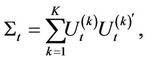
where is the transpose of the vector.

Ito’s lemma can be used to find a diffusion SDE for the process

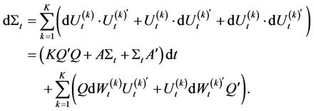
As it can be seen, the drift term of the SDE above contains, but the diffusion part contains the terms and separately. [1,3] show that also satisfies the following matrix SDE

where is an standard Brownian motion matrix.

2.1. The Dynamics of the Assets

The assets are defined on a probability space where is the information up to time and Q is the risk-neutral measure equivalent to the real-world measure P. Let’s assume that the firm’s asset price per share is given by. Here we review the results regarding the dynamics of the assets with stochastic covariance Wishart process. As before, assume the assets’ prices follow the multivariate real-world model

Here the vector is constant and is a symmetric positive definite matrix, the log-price process has the drift term

and the quadratic variation. Moreover, we assume that the Brownian motions driving the assets and the Brownian motions driving the Wishart process are uncorrelated. accounts for risk premium (under risk neutral measure). For the transition distribution of given and we have

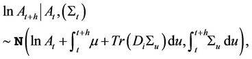
and the unconditional probability function can be found by Integration over the distribution function of.

Up to now we have described the dynamics of the assets’ prices with stochastic covariance structure coming from the Wishart process. The asset's price for a firm is not directly observed from the market. This leads us to structural credit risk models which introduce the equity as a form of a derivative on the asset of the company. Then the role of the model is in connecting the equity market to the default event. For example [3] proposes a dynamics for the assets and liabilities in the Merton’s model where the equity is defined as a call option on the asset with liability as the strike price. This is a direct extension of the Merton model with multivariate stochastic volatility. In that case the price of a bond has quasi closed-form formulas based on the closed formulas for the conditional Laplace transform of the joint price-covariance process. We prefer not to use this model for several reasons. First, we found the CreditGrades model more popular in financial markets because of its ability to link the structural framework to equity derivatives. On the other hand, the model proposed by [3] has one common Wishart process and one distinct Wishart processes for each asset. Therefore, the number of parameters for the model is high and the calibration is extremely illposed because of the high degree of freedom imposed by the number of parameters inside the model. We found that in the case of two companies, assuming only one Wishart process driving the covariance matrix gives a fairly flexible model to capture market’s behavior, while at the same time provides a fewer number of parameters.

Next, we introduce the equity process based on the CreditGrades’ perspective rather than Merton’s perspective taking advantage of the flexibility of the CreditGrades model. This will enrich the credit risk modeling with possibility of early default and also a straightforward link between credit risk and the equity market. We will derive a formula for the infinitesimal generator of the joint equity-covariance process below. This operator will play an important role in the partial differential equation of the equity option’s price.

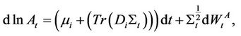
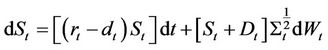
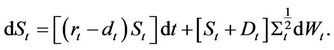
Now that we have identified the dynamics of the assets, we explain the mechanism of the CreditGrades model. As before, we assume that the firm’s value is driven by the dynamics

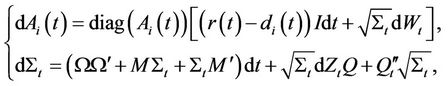(1)

where 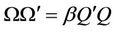for some and is a negative definite matrix. We assume that assets are driven by the Brownian motion, the covariance matrix of the assets which follows a Wishart process is driven by the Brownian motion and two Brownian motions and are uncorrelated. We assume that is the firm’s equity price per share, is the firm’s debt per share and is the firm’s recovery rate. has a deterministic growth rate, where is the risk free interest rate and is the dividend yield for the firm. The recovery part of the debt, , is the default barrier for the asset. Therefore, the default time based on CreditGrades model is given by

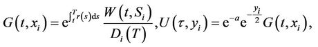
In the framework of CreditGrades model, the equity’s value is given by

In terms of the equity, the default time can be written as. Zero is an absorbing state for the equity process which makes the pricing of the equity option similar to pricing of down-and-out options studied by [11]. By using, the dynamics of and equation (1), the equity follows a shifted log-normal SDE. We will use the notation, and I denoting diagonal matrix and vector with elements and the matrix of ones respectively1.

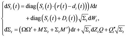(2)

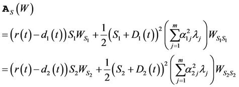
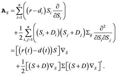
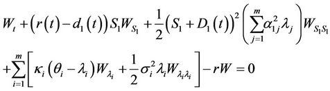
Note that the solution of the dynamics above can reach negative values but not before the stopping time. We force sufficient conditions on the Wishart process to make mean reverting. For our purposes, we assume is negative definite and for some. Moreover, without loss of generality, we assume. We first derive the infinitesimal generator of the joint process. This operator will appear in the pricing PDE for equity options and the probabilities of default in the next section Proposition 1: The infinitesimal generator of the joint process is given by

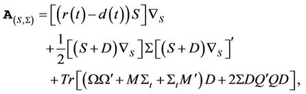
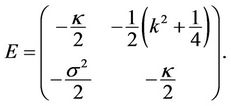
where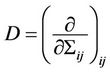, is the trace of a matrix, and we’ve used the notation 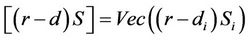and.

2.2. Derivative Pricing; Analytical Results

In this section, we tackle the pricing problem of our credit risk model. We will use the fourier transform and method of images to solve the pricing problem for European calls and puts on the equity

2.2.1. Equity Call Options

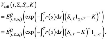
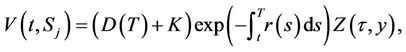
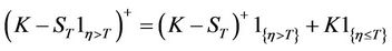
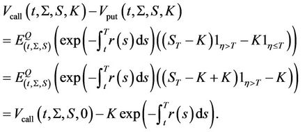
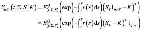
The price of a European Call option on the equity is calculated by discounting the risk-neutral expectation of the payoff at maturity. Since

the price of the call option could be rewritten as

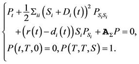
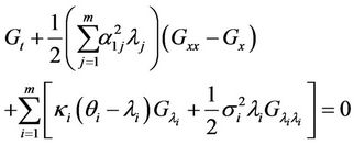
The price of a single name derivative on one of the equities satisfies the partial differential equation . Specially, the price of an equity call option is given by the PDE

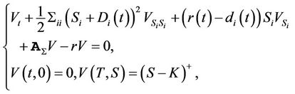(3)

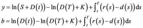
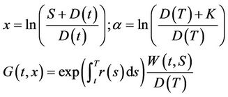
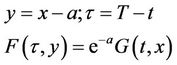
where is the infinitesimal generator of the joint process given by the proposition 1. We first change the variables by,

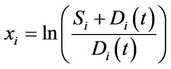and

to transform the PDE to

(4)

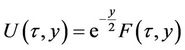
To use the method of images, we need to eliminate the drift term first, hence we change the variables by

, and.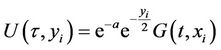

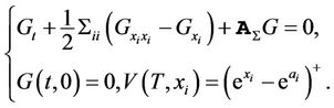
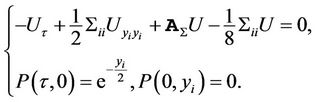
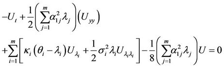
Then, PDE (3) transforms to

(5)

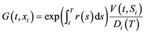
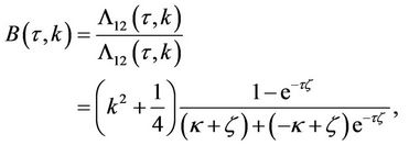
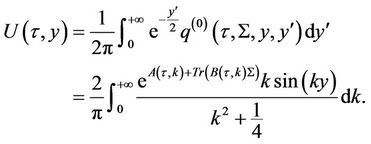
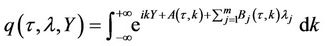
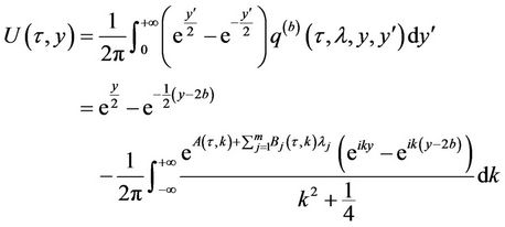
The PDE (5) is our reference PDE to solve the pricing problem for equity options on. We have the following proposition for the Fourier transform of the Green’s function of PDE Proposition 2: The Fourier transform of the Green’s function of PDE is given by

(6)

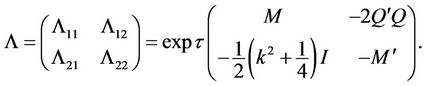
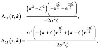
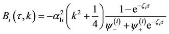
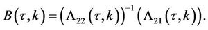
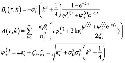
where

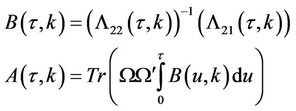
with

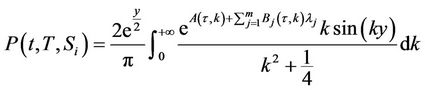
Now that we have found the Fourier transform of the Green’s function of the pricing PDE, we solve the pricing problem for an equity call option by the method of images.

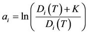
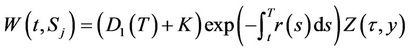
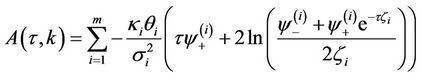
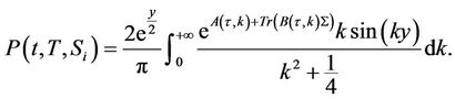
Proposition 3: The price of a call option on with maturity date and strike price is given by

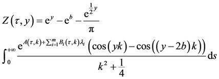
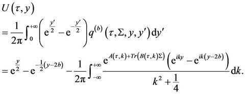
and the function is defined by

(7)

with and given as in proposition 2.

For large values of k, the integrand in (7) is exponentially decreasing which makes it easy to evaluate the integral numerically.

Remark 1: As we have mentioned before, our result covers [9] as a special case. If in the dynamics of the asset (1), we assume and for the parameters we let, and, propositions 2 and 3 yield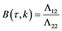. Now to find andby proposition 2 we have

is a matrix with

where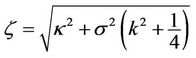. Therefore,

The function can be found by integration from. This gives the price of equity call option in the presence of Heston stochastic volatility (as in [9] Equations (3.5)-(3.7)).

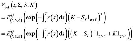
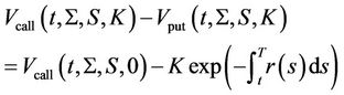
The price of a European put option on the equity is calculated by discounting the risk-neutral expectation of the payoff at maturity. Similarly to payoff of the call option, one can check that

. Therefore, the price of the put option could be rewritten as

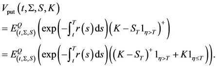(10)

Equations (3) and (10) give the put-call parity for the equity options

2.2.2. Survival Probabilities and Credit Default Swaps

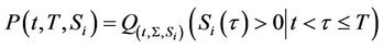
Suppose is the survival probability for the company

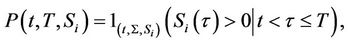
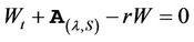
then using Feynman-Kac formula, satisfies the partial differential equation.

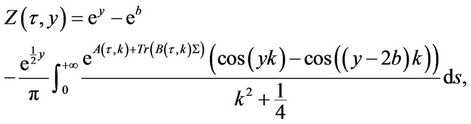
Proposition 4: The survival probability for the firm is given by

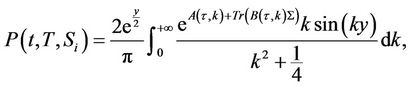
with functions and as in equation (7).

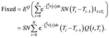
Credit default swaps are one of the most popular credit derivatives traded in the market. A CDS provides protection against the default of a firm, known as reference entity. The buyer of the contract pays periodic payments, called CDS spreads, until the default time or maturity date. In return, the seller of the CDS provides the buyer with the unrecovered part of the notional if default occurs. The valuation problem of a CDS is then to give the CDS spread a value such that the contract begins with a zero value. This means that the value of the floating leg and the fixed leg should coincide when the contract is written. Assume that the CDS spread is denoted by sp the periodic payments occur at, the notional is, the time of default is denoted by τ and the recovery rate is the constant. The fixed leg of the CDS is the value at time of the cash flow corresponding to the payments the buyer makes. With the above notation we have

(11)

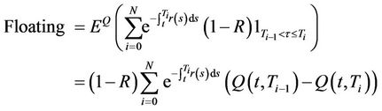
On the other hand, the floating leg, which is the value of the protection cash flow at, is

(12)

The CDS spread is chosen such that the contract has a fair value at. By setting the fixed leg equal to the floating leg, the equations and imply

3. The CreditGrades Principal Component Model

In this section, we first present an stochastic eigenvalue process which is used for the covariance of the assets process. The section then covers pricing of derivatives using the CreditGrades model. We first remind the formal definition below:

Definition 2: The instantaneous stochastic covariance follows a Principal Component Model if:

(13)

where is a diagonal matrix whose elements are real valued CIR process defined, for, by:

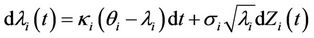(14)

the’s are independent one-dimensional Brownian motion and is an orthogonal constant matrix. We also assume, for andwithout lost of generality,.

The main ingredient of this multivariate process is a family of one-dimensional stochastic processes for the eigenvalues. We assume for simplicity Heston-type processes but this approach works for other kind of processes.

The conditions, ensure stationarityergodicity and mixing conditions for the one-dimensional processes (see [4]). The constraints 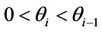ensure that the eigenvalues process will keep, on average, the same order but their paths could eventually cross over. This ordering on average allows us to keep the eigenvalues with greatest mean reverting levels while dropping the less significant ones.

3.1. The Dynamics of the Assets

We assume that the firm’s value is driven by the dynamics

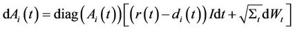
where, , with

Each follows a CIR process of the type

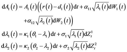
In the two assets case, the above dynamics follows

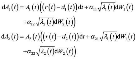(15)

where the eigenvalues of the covariance process follow

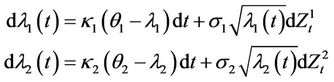
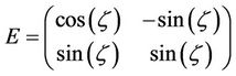
And assuming as the angle that the first eigenvector makes with the real axis, the eigenvector matrix is given by

We assume that assets are driven by the Brownian motion, the covariance matrix of the assets is driven by the Brownian motion and two Brownian motions and are uncorrelated. The reason we make the independence assumption between stock and its volatility is that closed form formulas for the value of double-barrier options and equity options are not available when the asset and its volatility are correlated as pointed out by [8, 9].

The infinitesimal generator of the joint process, , appears in the pricing PDE. Here we find a fomula for this operator to use it for our pricing purposes in the next section. Since, the equity satisfies the stochastic differential equation

can be divided into three terms related to the stock’s operator, the covariance operator and their joint operator

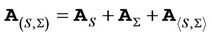
Since and are independent, the last term is zero. From the dynamics of the equity, we know that

(16)

And from the classical results regarding the infinitesimal generator of the CIR process

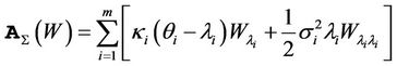
Therefore, if is a derivative on the first underlying asset only, we have

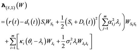
In the next section, we derive closed formulas for the price of equity options and marginal probabilities of default.

3.2. Derivative Pricing; Analytical Results

In a model with two underlyings, the first asset follows the following process:

We will show next the prices of several derivatives as seen from a credit perspective.

3.2.1. Equity Call Options

Calculating equity option prices is essential to calibrate the stochastic correlation CreditGrades model since this model uses the information available from the equity options to estimate the parameters of the model. Later, we will use the evolutionary algorithm method to match the theoretical results of our extended CreditGrades model with the market data. One of the advantages of the CreditGrades model compared to Merton’s model, is the straight forward link it makes with the equity option markets. The price of the equity option can be calculated by discounting the payoff function at the maturity. The only subtle point here in pricing these options lies in the specific dynamics of the equity itself and the possibility of default for the company. In Black-Scholes model, the stock follows geometric Brownian motion which is a strictly positive process with a log-normal distribution and never hits zero. In the CreditGrades model, equity is modeled as a process satisfying a shifted log-normal distribution which hits the state zero when the company defaults. Because of the absorbing property of the state zero for the equity process, there is a resemblance in pricing the equity options and the pricing of the downand-out options. By considering the barrier condition for equity, the payoff of an equity call option is given by

. Therefore the price of an equity call option can be written as:

Similarly, the payoff of an equity put option is. Therefore, the price of an equity put option is given by:

Equation (18) give the put-call parity for the equity options:

(18)

The following proposition gives a closed form solution for the price of an equity call option on the first asset. Proposition C5 and equation (18) give the price of an equity put option. This result is an essential tool to calibrate the model in the next section.

Proposition 5: The price of a call option on with maturity date and strike price is given by:

with

3.2.2. Survival Probabilities and Credit Default Swaps

Similar techniques can be used to find the marginal probabilities of default. Suppose is the survival probability for the company

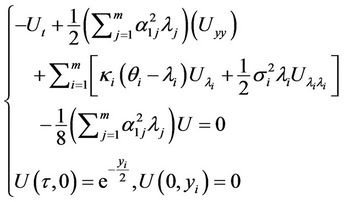
Using the Feynman-Kac formula, satisfies the partial differential equation with boundary conditions and. We have the following proposition for the survival probabilities Proposition 6: The survival probability for the firm is given by

Knowing the probability of the default, one can find the CDS spread for the underlying company. Assume that the CDS spread is denoted by, the periodic payments occur at, the notional is, the time of default is denoted by and the recovery rate is the constant. The fixed leg of the CDS is the value at time of the cash flow corresponding to the payments the buyer makes. With the above notation we have

On the other hand the floating leg, which is the value of the protection cash flow at, is

The CDS spread is chosen such that the contract has a fair value at. By setting the fixed leg equal to the floating leg, the Equation (18) imply

4. Conclusion

We presented a structural credit risk model which considers stochastic correlation between the assets of the companies. The stochasticity of the volatility and correlation comes from first a Wishart process and then a principal component stochastic covariance process which drives the covariance matrix of the assets. To model credit risk, we use the so called CreditGrades model. Using the affine properties of the joint log-price and volatility process, we solved the pricing problem of the equity options. We used our analytical techniques to derive quasi closed-form solution for equity options, probabilities of defaults and prices of CDSs issued by the companies.

REFERENCES

Appendix

Proof proposition 1:

Since

can be divided into

Since and are independent, the last term is zero. By [1]:

To find, by the dynamics of

Proof proposition 2:

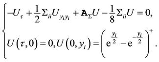
Define 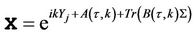and substituting into (5) yields

(19)

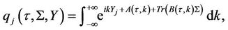
Note that the functions satisfying the ODE above (i.e. and) do not depend on the variable. So we set to get

(20)

and then by substituting (20) into (19) leads to 

To solve the above ODE, we rearrange the equation as

Therefore, satisfies:

Since the function is independent of, assuming to be a zero matrix except for the entry. Therefore

(21)

This matrix Ricatti equation has been studied in the literature (see [13]) and in Affine term structure models (see [14]) leading to:

can be found by integration.

Proof proposition 3:

The previous proposition gives the Fourier transform of the Green’s function of the pricing PDE. Now note is invariant with respect to the change of variables and, therefore is an even function with respect to. This implies that the Fourier transform of the Green’s function absorbed at is

By Duhamel’s formula

With the consequent changes of variables

one can conclude that.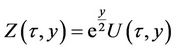

Proof Proposition 4:

The PDE for survival probability is:

(22)

Using the change of variables,

and, the PDE transforms to

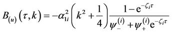
This PDE is the same as (5). In Proposition 2, we have proved that the aggregated Green’s function for this PDE is of the form (28). To find a bounded solution reflected at, we use the method of images to write the absorbed aggregated Green’s function as

Now by Duhamel’s formula

Using the change of variable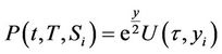, one can find the survival probability from the above formula for as:

Proof proposition 5:

By risk neutral valuation, W satisfies

where is the infinitesimal generator of the SDE driving the equity. By substitution

From now, we drop the index. We change the variables as

which gives

We perform the second change of variables as

And finally we perform the third change of variables

leading to

We claim that the Fourier transform of the Green’s function for the above PDE is of the form

(23)

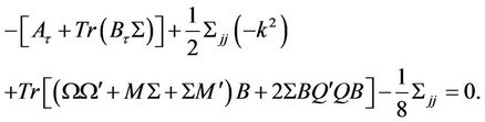
We know that satisfies the corresponding PDE. Plugging into the PDE, one gets Ricatti ODE’s for and’s, which finally gives the function as

The representation for the function comes from equation

Note that has a structure invariant with respect to the change of variables

Therefore, the Fourier transform absorbed at is

the above expression and Duhamel’s formula leads to:

Since the result follows.

Proof proposition 6:

Substituting for the infinitesimal generator from Equation (17), solves

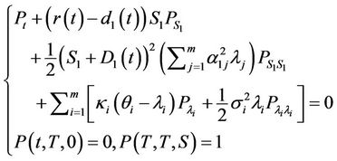(26)

Using the change of variables,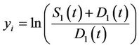

and, the PDE (26) transforms to

In the proof of the proposition 5 we showed that the Fourier transform of the Green’s function for the above PDE is of the form

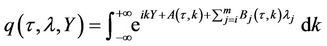
and the functions and are given. In order to find a bounded solution reflected at, we use the method of images to write the absorbed aggregated Green’s function as

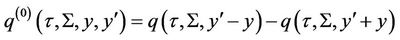
Now by the Duhamel’s formula

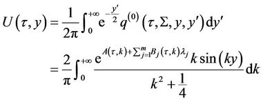
Therefore, the survival probability is given by

NOTES

¹Note that with the above dynamics is allowed to gain negative values but not prior to the stopping time. Even though it might seem unreasonable to allow have negative values, this doesn’t affect any of the pricing formulas since whenever the process is involved, it is followed by the truncating factor ( as in Equations (3) and (10) for the payoffs of call and put options.)

REFERENCES

- M.-F. Bru, “Wishart Processes,” Journal of Theoretical Probability, Vol. 4, No. 4, 1991, pp. 725-751.
- M. Escobar, B. Gotz, L. Seco and R. Zagst, “Pricing of a CDO on Stochastically Correlated Underlyings,” Quantitative Finance, Vol. 10, No. 3, 2007, pp. 265-277.
- C. Gourieroux, J. Jasiak and R. Sufana, “Derivative Pricing with Multivariate Stochastic Volatility: Application to Credit Risk,” Working Paper, 2004.
- C. Gourieroux and R. Sufana, “The Wishart Autoregressive Process of Multivariate Stochastic Volatility,” Econometrics, Vol. 150, No. 2, 2009, pp. 167-181. doi:10.1016/j.jeconom.2008.12.016
- J. DaFonseca, M. Grasselli and F. Ielpo, “Estimating the Wishart Affine Stochastic Correlation Model Using the Empirical Characteristic Functionk,” Working Paper ESILV, RR-35, 2007.
- J. DaFonseca, M. Grasselli and C. Tebaldi, “A Multifactor Volatility Heston Model,” Quantitative Finance, Vol. 8, No. 6, 2006, pp. 591-604.
- J. DaFonseca, M. Grasselli and C. Tebaldi, “Option Pricing When Correlations Are Stochastic: An Analytical Framework,” Review of Derivatives Research, Vol. 10, No. 2, 2007, pp. 151-180.
- A. Lipton, “Mathematical Methods for Foreign Exchange: A Financial Engineers Approach,” World Scientific, Singapore, 2001.
- A. Sepp, “Extended Creditgrades Model with Stochastic Volatility and Jumps,” Wilmott Magazine, 2006, pp. 50- 62.
- S. L. Heston, “A Closed-Form Solution for Options with Stochastic Volatility, with Applications to Bond and Currency Options,” Review of Financial Studies, Vol. 6, No. 2, 1993, pp. 327-343. doi:10.1093/rfs/6.2.327
- R. C. Merton, “On the Pricing of Corporate Debt: The Risk Structure of Interest Rates,” Journal of Finance, Vol. 29, No. 2, 1974, pp. 449-470.
- R. Stamicar and C Finger, “Incorporating Equity Derivatives into the Creditgrades Model,” RiskMetrics Group, Tampa, 2005.
- H. Abou-Kandil, G. Freiling, V. Ionescu and G. Jank, “Matrix Riccati Equations in Control and Systems Theory,” Springer, Berlin, 2003. doi:10.1007/978-3-0348-8081-7
- M. Grasselli and C. Tebaldi, “Solvable Affine Term Structure Models,” Mathematical Finance, Vol. 18, No. 1, 2004, pp. 135-153.