Journal of Mathematical Finance
Vol.2 No.3(2012), Article ID:22126,5 pages DOI:10.4236/jmf.2012.23026
Credit Constraints and Decisions in Exports: Theory under Asymmetric Information
Key Laboratory of International Commodity Transaction Analysis and Simulation, Liaoning University of International Business and Economics, Dalian, China
Email: xiongyingsharon@sina.com
Received January 19, 2012; revised February 20, 2012; accepted March 3, 2012
Keywords: Credit Constraints; Asymmetric Information; Heterogeneous Productivity
ABSTRACT
This paper examines why credit constraints for domestic and exporting firms arise in a setting where banks do not observe firms’ productivities. To maintain incentive-compatibility, banks lend below the amount needed for first-best production. The longer time needed for export shipments induces a tighter credit constraint on exporters than on purely domestic firms, even in the exporters’ home market. Greater risk faced by exporters also affects the credit extended by banks. Extra fixed costs reduce exports on the extensive margin, but can be offset by collateral held by exporting firms.
1. Introduction
The financial crisis of 2008 has led researchers to ask whether credit constraints faced by exporters played a significant role in the fall in world trade. There are a wide range of answers: Amiti and Weinstein (2009) argue that trade finance was important in the earlier Japanese financial crisis of the 1990s, and Chor and Manova (2010) find that financially vulnerable sectors in source countries did indeed experience a sharper drop in monthly export to the United States. In contrast, [1] find no evidence that trade credit played a role in restricting imports or exports for the recent episode in the US, while for Belgium, Behrens, Corcos and Mion (2010) argue that to the extent that financial variables impacted exports, they also impacted domestic sales to the same extent. Of course, the potential causal link between financial development and international trade at country level was recognized long before the recent crisis. For example, Kletzer and Bardhan (1987; see also Qiu, 1999, Beck, 2002, and Matsuyama, 2005) argued that credit-market imperfections would adversely affect exporters needing more. nance and hence in. uence trade patterns. That theme was picked up in a Melitz (2003) model by Chaney (2005), and implemented by Manova (2008), who argue that credit constraints affect exporting firms in different countries and industries differently due to fixed costs.
The key feature of our model is that the bank has incomplete knowledge of firms, in two respects. First, the bank cannot observe the productivity of firms. We believe this assumption is realistic in rapidly growing economies such as China with rapid entry, and perhaps more generally. The bank will confront firms with a schedule specifying the amount of the loan and the interest payments to maximize its own profits. From the revelation principle, without loss of generality we can restrict attention to schedules that induce firms to truthfully reveal their productivity. Second, the bank cannot verify whether the loan is used to cover the costs of production for domestic sales or for exports. This second assumption means that we are not really modeling the loans from the bank as “trade finance”: such loans would typically specify the names of the buying and selling party, so the bank could presumably verify whether the loan was for exports or not. Rather, the loans being made by the bank are for “working capital” to cover the costs of current production, regardless of where the output is sold. The assumption that banks cannot follow a loan once the money enters the firm is made in a different context.
With these assumptions, in section 2 we derive the incentive-compatible loan schedule by the bank that maximizes its own profits. [2] argue that sales revenue of firms is less than would occur in the absence of any working-capital needs, i.e. the incentive-compatible loans impose credit constraints on firms. [3] find that the reason for these credit constraints is that a firm suffers only a second-order loss in profits from producing slightly less than the first-best and borrowing less from the bank, but obtains a first-order gain from reducing its interest payments in this way. So a firm that is not credit constrained will never reveal its true productivity and borrow enough to produce at the first-best. Hence, incentive-compatibility requires that the firm is credit constrained. Furthermore, because banks cannot follow a loan once it enters the firm, the credit constraint applies to the exports and domestic sales of a firm engaged in both these activities, which we refer to as an exporting firm. Because exports take longer in shipment, such exporting firms face a tighter credit constraint on both markets than purely domestic firms.
So our answer to the question “is credit for exports and domestic sales treated differently?” is nuanced: when these activities occur in the same firm, the bank treats them equally; but when these activities occur in an exporting firm and a purely domestic firm respectively, they are indeed treated differently. The tighter credit constraint on exporting firms comes from the first reason for exports to be treated differently than domestic sales and reduces exports on the intensive and extensive margins. The second reason, greater risk, arises due to the risk of a firm not being paid for the default risk of the firm not repaying the bank. We find that higher default risk for exporters raises their interest payments for any given loan, acting in a similar manner to credit constraints. The third reason, which is the extra fixed costs faced by exporters, reduces the extensive margin of exports.
2. Incentive-Compatible Loans
We suppose there are two countries, home and foreign (henceforth foreign counterparts of the variables are denoted with an asterisk *). Labor is the only factor for production and the population is of size L at home. There are two sectors, where the first produces a single homogeneous good that is freely traded and chosen as numeraire, this assumption is the same as [4]. Each unit of labor in this sector produces a given number of units of the homogeneous good. We assume that both countries produce in this sector and it follows that wages are thus fixed by the productivity in this sector. The second sector produces a continuum of differentiated goods under monopolistic competition.
2.1. Consumers’ Decision
Consumers are endowed with one unit of labor and the preference over the differentiated good displays a constant elasticity of substitution. The utility function of the representative consumer is
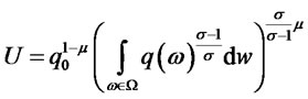


where  denotes each variety,
  is the set of varieties available to the consumer,
  is the constant elasticity of substitution between each variety, and
  is the share of expenditure on the differentiated sector. The aggregate price index in the differentiated sector is:
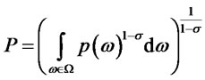 (1)
(1)
where  is the price of each variety. Accordingly, the demand for each variety is:
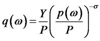 (2)
(2)
where  is the total expenditure on the differentiated good at home.
2.2. Domestic Firms’ Decision
Under incomplete information, the bank does not observe the productivity level x of a firm coming to it for a loan. In order to maximize profits, the bank will design a schedule of loans  and interest payments
  contingent on the announced productivity level
 . If the firm defaults, which occurs with probability
 , we follow Manova (2008) in assuming that the bank can collect the collateral amount,
 .
.
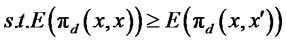
By the revelation principle, the bank can do no better than to design a loan-interest payment schedule that induces firms to reveal their true productivity [5], . Adding this incentive compatibility condition as a constraint, the domestic firms profit maximization problem is:
 (3)
(3)
and also subject to the domestic demand function in (2). In this problem, the firm pays the fraction  of costs with certainty, while borrowing for the remainder and repaying with probability
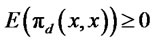
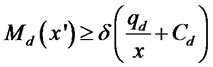
 . The first constraint is the incentive compatibility constraint [6], and the second ensures that expected profits are non-negative, and the third specifies that the amount of the loan must cover the fraction
  of fixed and variable costs at the chosen production level
 .
.
The third constraint above will be binding in equilibrium, which implies:
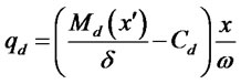 (4)
(4)
Provided that the loan and interest payment schedules are differentiable in , then the incentive-compatibility condition implies that,
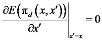 (5)
(5)
By substituting the quantity Equation (4) into the demand function (2) we solve for the price. Using that we derive the firms profits , and take the derivative as in (5) to obtain:
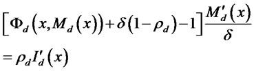 (6)
(6)
where
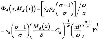 (7)
(7)
The value of  on the first line of (7) is recognized as the ratio of expected marginal revenue to marginal costs. A firm facing the project risk of
  but without any need to borrow will produce where
 , while a firm that produces less due to insufficient loans will have
 . This means that
  is a measure of firm’s credit constraint, and the larger is
  then the lower is the quantity produced due to this constraint. The second line of (7) is obtained by using the quantity in (4) and solving for the corresponding price from demand (2). It is apparent that having lower loans
  will raise
 , indicating that the credit constraint is tightened.
We can now develop some intuition as to why the bank might need to impose credit constraints. Let us suppose that the bank lends more to higher productivity firms, and also collects more in interest payments: we will confirm that these monotonicity conditions hold in the optimal schedules for the bank. Then in (6), both  and
and  are positive. It follows that the expression in brackets on the left must be positive, so in the no-default case where
  it follows that the firm must be credit constrained, i.e.
 . Following [6], the reason this condition needed is that a firm that is producing at the first-best with marginal revenue equal to marginal cost would have only a second-order loss in profits from announcing a slightly smaller productivity
 , and producing slightly less. But the firm would have a first-order gain from the reduction in interest payments
 . So a firm at the first-best would always understate its productivity, and it follows that a credit constraint is needed to ensure incentive compatibility. We will formalize this intuition below, and show that
  even in the presence of default.
2.3. Exporters’ Decision
Following the thought of [7], we assume that the monopolistic bank cannot enforce different contracts to separate loans for domestic market and export market. Rather, exporters are free to determine how to allocate the loan to both markets. In comparison with purely domestic firms, exporters have three differences:
1) Longer time needed to pay back their export loans  (which enters the bank’s problem analyzed in the next section); 2) Potentially greater project risk,
 ; and default risk,
  , where we assume that the default risk for the exporter applies to the total loan from the bank; 3) Additional fixed costs of exporting, which are denoted by
 .
.
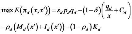
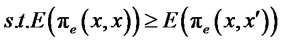
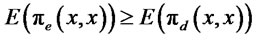
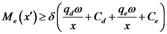
An exporter chooses quantities to produce at domestic market and export market and claims a productivity to maximize its expected profit:
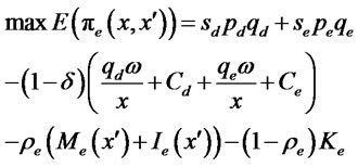 (8)
(8)
and subject to export demand,
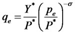 (9)
(9)
where  is the foreign total expenditure on the differentiated good. The total loan received by the exporter is denoted by
  and total interest payments are
 , while
  is the exporter’s total collateral.
The first two constraints above are analogous to those for the domestic firm, but the third constraint is different and important. It states that the total amount of the loan given to the exporter must cover the working-capital needs of both domestic and export production costs. From the exporting firm’s perspective, these funds are fully fungible so the bank is making a single loan. The conclusion is the same as [8]. Likewise, the bank will receive a single interest payment, which is  in expected value.
Setting up a Lagrangian with the objective function and the third constraint, and solving this problem for the choice of  and
and , it is readily shown that the firm will maximize its profit by choosing quantities in the two markets such that:
 (10)
(10)
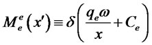
This condition states that the loan will be allocated within the firm so that expected marginal revenue in the domestic and export markets are equalized. It means that for any given loan, the bank will know exactly how production is allocated between the two markets. Thus for notational convenience, we break up the total loan  into the component intended to cover domestic costs
 , and the component intended to cover export costs
 . That is, for any announcement of productivity
 , and subsequent choice of quantities satisfying (10), we will define the loans allocated to each market as,
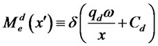 (11)
(11)
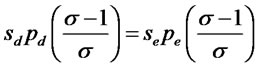
We can readily solve for this allocation of loans by subtracting fixed costs from both sides of (11) and taking the ratio. Then using demand in (2) and (9), combined with the requirement from (10) that the expected prices  and
and  are equalized, it follows that the loans to the two markets are related by:
 (12)
(12)
where we define the shares of demand coming from the domestic and foreign markets as:
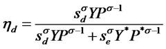 (13)
(13)
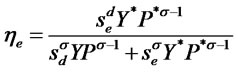
We see from (12) that there is a simple, linear relationship between the loans allocated to the two markets. We can now proceed analogously to the domestic firms’ problem. We use (11) to determine the quantity sold in each market analogous to (4), depending on the loans  and
and , and substitute into demand (2) and (9) for each market to determine prices. With these we obtain the firms’ profits
 . Taking the derivative of expected profits with respect to
 , and setting that equal to zero, we obtain the condition for incentive compatibility:
 (14)
(14)
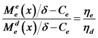
where,
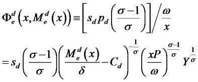 (15)
(15)
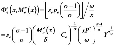
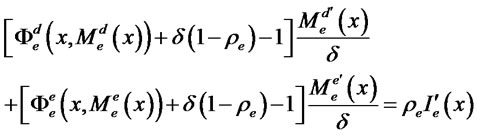
and from the equality of expected marginal revenues in (10) we have that,
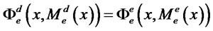 (16)
(16)
The interpretation of these conditions is analogous to what we obtained for domestic firms. The values  and
and  are the ratio of expected marginal revenue to marginal costs in the two markets served by the exporter. Credit constraints would mean that
  and
and , so the firm would be selling less in both markets than would be optimal in the absence of any risk or constraints. We now determine the magnitude of credit constraints that are optimal for the bank.
2.4. Bank’s Decision
We do not assume that the bank can identify domestic firms and exporters, but only observes the announced productivities of firms. As in the Melitz (2003) model, firms will enter into domestic production and export based on the profitability of these activities. This means that the cutoff domestic firm with productivity  is defined by the zero-cutoff-profit condition
 , and the cutoff exporter with productivity
  by the condition
 . These cutoff productivities can differ from in the Melitz (2003) model, of course, because here they are influenced by the credit conditions offered by banks. A standard property of firm profits under any incentive-compatible policy is that they must be non-deceasing in the true productivity, i.e.
  and
and  are non-decreasing in
 . We will identify additional conditions below needed to ensure that the cutoff exporter, in particular, is well defined.
The monopolistic bank chooses the loans given to domestic firms subject to the incentive-compatibility condition (6), and chooses the loans given to exporters for the domestic market  and for export market
 , subject to the incentive-compatibility conditions (14) and the equality of marginal revenue (16). The bank’s problem is then to choose
 ,
,  ,
,  ,
,  and
and  to maximize its profits:
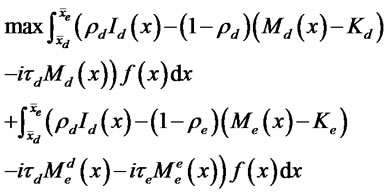 (17)
(17)
s.t. (6) if  and (14) and (16) if
where  is the opportunity cost of lending the loan for one unit of period and
  and
and  are the length of the periods that the firm has to hold the loans in the domestic and export market respectively, as defined earlier. The probability density function of firms’ productivity distribution is
 .
.
3. Conclusion
In this paper, we have asked why firms will face credit constraints on their domestic sales and exports. We rely on the idea that firms must obtain working capital prior to production and that their productivity is private information. From the revelation principle, the bank can do no better than to offer loan and interest schedule that lead the firms to truthfully reveal this information. We argue that such incentive-compatible schedules will lead to credit constraints on the firms. The reason for this is that a firm that is not credit constrained would suffer only a second-order loss in profits by producing slightly less and borrowing less, but would have a first-order reducetion in interest payments. Thus, such a firm would never truthfully reveal its productivity and produce at the firstbest.
4. Acknowledgements
I thank an anonymous referee for the comments and suggestions.
REFERENCES
- J. Levinsohn and A. Petrin, “Estimating Production Functions Using Inputs to Control for Unobservable,” Review of Economic Studies, Vol. 70, No. 2, 2003, pp. 317-341. doi:10.1111/1467-937X.00246
- P. Bolton and D. S. Scharfstein, “A Theory of Predation Based on Agency Problems in Financial Contracting,” American Economic Review, Vol. 80, No. 1, 1990, pp. 93-106.
- G. L. Clementi and H. A. Hopenhayn, “A Theory of Financing Constraints and Firm Dynamics,” Quarterly Journal of Economics, Vol. 121, No. 1, 2006, pp. 229- 265.
- D. Greenaway, A. Guariglia and R. Kneller, “Financial Factors and Exporting Decisions,” Journal of International Economics, Vol. 73, No. 1, 2007, pp. 377-395. doi:10.1016/j.jinteco.2007.04.002
- C. Holz, “China’s Statistical System in Transition: Challenges Data Problems, and Institutional Innovations,” Review of Income and Wealth, Vol. 50, No. 3, 2004, pp. 381-409. doi:10.1111/j.0034-6586.2004.00131.x
- W. Keller and S. R. Yeaple, “Multinational Enterprises, International Trade, and Technology Diffusion: A FirmLevel Analysis of the Productivity Effects of Foreign Competition in the United States,” Review of Economics and Statistics, Vol. 91, No. 4, 2009, pp. 821-831. doi:10.1162/rest.91.4.821
- L. D. Qiu, “Credit Rationing and Patterns of New Product Trade,” Journal of Economic Integration, Vol. 14, No. 1, 1999, pp. 75-95.
- I. Murtazashvili and J. M. Wooldridge, “Fixed Effects Instrumental Variables Esimation in Correlated Random Coefficient Panel Data Models,” Journal of Econometrics, Vol. 142, No. 1, 2008, pp. 539-552. doi:10.1016/j.jeconom.2007.09.001