Open Journal of Ecology
Vol.3 No.2(2013), Article ID:30967,7 pages DOI:10.4236/oje.2013.32013
Predicting nesting habitat of Northern Goshawks in mixed aspen-lodgepole pine forests in a high-elevation shrub-steppe dominated landscape
![]()
1Raptor Research Center, Department of Biological Sciences, Boise State University, Boise, USA; *Corresponding Author: RobertMiller7@u.boisestate.edu
2Idaho Bird Observatory, Department of Biological Sciences, Boise State University, Boise, USA
3Minidoka Ranger District, Sawtooth National Forest, USDA Forest Service, Burley, USA
Copyright © 2013 Robert A. Miller et al. This is an open access article distributed under the Creative Commons Attribution License, which permits unrestricted use, distribution, and reproduction in any medium, provided the original work is properly cited.
Received 23 December 2012; revised 24 January 2013; accepted 12 February 2013
Keywords: Accipiter gentilis; Breeding Ecology; Habitat; Idaho; Nest Model; Northern Goshawk
ABSTRACT
We developed a habitat suitability model for predicting nest locations of breeding Northern Goshawks (Accipiter gentilis) in the high-elevation mixed forest and shrub-steppe habitat of south-central Idaho, USA. We used elevation, slope, aspect, ruggedness, distance-to-water, canopy cover, and individual bands of Landsat imagery as predictors for known nest locations with logistic regression. We found goshawks prefer to nest in gently-sloping, east-facing, non-rugged areas of dense aspen and lodgepole pine forests with low reflectance in green (0.53 - 0.61 µm) wavelengths during the breeding season. We used the model results to classify our 43,169 hectare study area into nesting suitability categories: well suited (8.8%), marginally suited (5.1%), and poorly suited (86.1%). We evaluated our model’s performance by comparing the modeled results to a set of GPS locations of known nests (n = 15) that were not used to develop the model. Observed nest locations matched model results 93.3% of the time for well suited habitat and fell within poorly suited areas only 6.7% of the time. Our method improves on goshawk nesting models developed previously by others and may be applicable for surveying goshawks in adjacent mountain ranges across the northern Great Basin.
1. INTRODUCTION
Habitat sets the ultimate limit on the success and distribution of any wild species [1]. It follows that many techniques have been developed to analyze relationships between habitat features and species distributions. Species habitat relationships are analyzed to predict the range of a species [2], to predict a species response to habitat change [3], to evaluate suitability of an environment to support species re-introduction [4], or to aid in the search for presence of a species [5,6]. A habitat distribution model or habitat suitability model relates the geographical distribution of species or communities to their present environment [7]. Techniques for the development of these models have ranged from using detailed field measurements [8] to the use of Geographic Information Systems (GIS) with remotely sensed data and sophisticated statistical procedures [5,7].
The choice among various analysis techniques depend upon the objectives of the work and the scale of the inference required. In using habitat suitability models, a mismatch between the scale of the data and the scale of the inference can lead to significant bias in the result [9]. Habitat selection patterns at a large scale can often disappear or change as the scale is reduced [10]. Additionally, the application of habitat models generated from data in one area may not readily apply to another area, especially if the model must be extrapolated beyond the range of data used to build the model [11,12].
The Northern Goshawk (Accipiter gentilis; hereafter “goshawk”) is a generalist predator occupying boreal and temperate forests of the Holarctic [13]. Studies have shown that goshawks prefer to nest in mature dense canopy cover with an open understory, often near water, with a gentle north or east aspect [14-17]. In addition, goshawks have been shown to nest in stands where heterogeneity is low [16,17] and nests are remote from human disturbance [18]. Lõhmus [19] found forest structure to be a more important influence than disturbance. The goshawk exhibits regional variation with its habitat use [5,14-16]. To better understand this variation and to ensure the proper scale of inference, regional analyses are warranted.
We developed habitat suitability models to quantify the habitat needs of goshawks in the unique environment of the South Hills and to aid in prioritizing areas to be searched for occupancy by nesting goshawks. Searching for nesting structures of goshawks is an expensive process [20]. Significant time can be spent accessing and searching low quality habitat. A high quality prediction model can significantly aid the search effort by increasing search efficiency. Our model will be useful for forest management and future surveying activities within the area and across the northern Great Basin where similar habitat exists.
2. METHODS
2.1. Study Area
We conducted this study in the South Hills encompassing the Cassia section of the Minidoka Ranger District of the Sawtooth National Forest in south-central Idaho (41.98˚ - 42.33˚N, 113.98˚ - 114.48˚W; Figure 1). The section occupies portions of Twin Falls and Cassia counties. The Cassia section contains approximately 125,000 hectares and is bordered primarily by Bureau of Land Management lands [21]. The naturally-fragmented forest is dominated by grasslands and mountain big sagebrush (Artemisia tridentata vaseyana; approximately 80%) [22]. The remaining forested landscape consists predominantly of aspen (Populus tremuloides), lodgepole pine (Pinus contorta), and sub-alpine fir (Abies lasiocarpa) [22].
2.2. Goshawk Nests
We discovered goshawk nests by searching historical
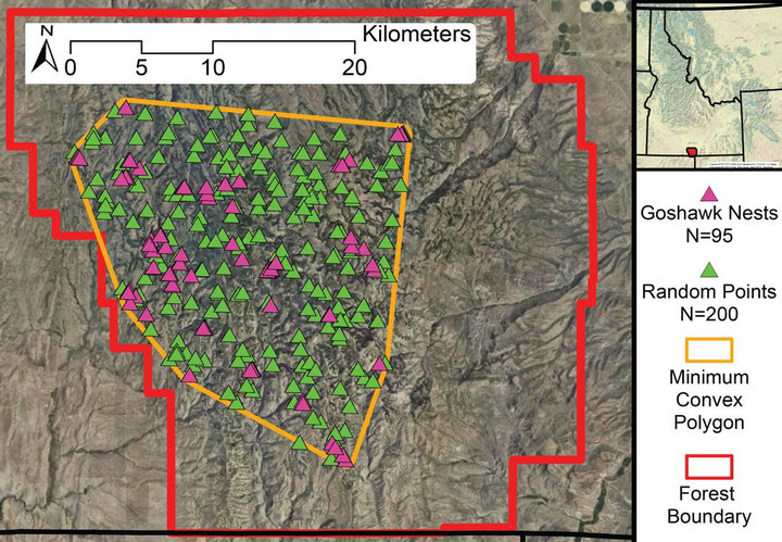
Figure 1. Cassia Section, Minidoka Ranger District, of the Sawtooth National Forest in south-central Idaho with known goshawk nest locations, 500-meter buffered minimum convex polygon (MCP) around known nest locations, and 200 randomly selected points constrained by MCP.
nesting territories provided by the Forest Service and additional areas prioritized through geographic information system analysis (Figure 1) [5,23]. We searched for nests by first checking historical nesting structures for occupancy, then searching on foot within a 300-meter radius of historical nesting structures for new nests. When no nests were found by these means, we then broadcasted alarm calls every 300 meters out to 1370 meters (588-hectare area) from historical nest structures to solicit a response [24]. We used an average male home range of 588 hectares that was previously established in the same study area [25]. Nest structures were discovered during the formal search process in addition to accidental discovery while we were in the area for other purposes. We randomly reserved 15% of the nest locations for a validation dataset and excluded these from model creation. Nest locations were classified by nesting substrate—aspen or lodgepole pine—to enable a unified analysis in addition to separate analyses by forest type.
We generated a minimum convex polygon encompassing a 500-meter buffer around all discovered nest structures (Figure 1). We generated 200 random points within this polygon to serve as control points for the habitat analysis (Figure 1). We made no effort to check these locations for nest structures or to limit their position relative to known nest locations. As a result our data set represented presence only data, with implied but not true absence. Furthermore, we did not assign substrate values to the random points, using the same control points for the overall analysis, aspen only analysis and lodgepole pine only analysis.
2.3. GIS Data
We acquired Digital Elevation Model (DEM) data from Inside Idaho at a resolution of 30 meters [26]. We calculated slope and aspect from the digital elevation model. We transformed aspect into two variables, northness and eastness, through trigonometric transformations [27]. We generated a ruggedness index using the relative position method [28]. Ruggedness is a measure of local elevation differences within a 330-meter roving window. Lower values represent nest trees located at or near the local minimum elevation. We acquired canopy cover data from the National Land Cover Database [29] and stream location data from Inside Idaho [30].
We acquired Landsat 7 Enhanced Thematic Mapper Plus (ETM+) imagery via ESRI’s Global Land Survey 2010 dataset [31]. The Landsat data included bands 1, 2, 3, 4, 5 and 7, was corrected for Scan Line Corrector (SLC) errors, and was enhanced with radiometric correction and histogram stretching to make it more visually appealing [31].
We used the stream data to create a 30-meter resolution raster file representing the distance of each pixel from the nearest water source. The distance-to-water layer and each of the Landsat image layers were resampled using bilinear interpolation to match the alignment of the digital elevation model. We did not include a measure of disturbance as not all of our nest structures were discovered using a random sample process and thus our dataset may be spatially biased toward human access. All raster layers were placed into a “raster stack” to aid in data management [32].
2.4. Statistical Analysis
We extracted data from each raster layer for each of our nests and random points. We used logistic regression to generate a model using elevation, slope, northness, eastness, ruggedness, canopy cover, distance-to-water, and each of the six Landsat image layers as predictors for nest presence. We selected the final predictor variables by using both backwards and forwards stepwise selection via AIC [33]. We verified the absence of multicollinearity in the final model using a Pearson correlation test with a threshold of 0.70. The resulting top model was recombined with the raster data block to generate a prediction layer for the study area.
We evaluated spatial autocorrelation of nest structures and occupied nest structures using the habitat model residuals and nest coordinates to calculate the Geary’s C statistic [34]. A Geary’s C value < 1 indicates clustered resources, whereas a value > 1 implies spatial regularity, and values near one imply a random distribution with no auto-correlation [34].
We reclassified the prediction layer into three categories—poorly suited, marginally suited and well suited— by first using a quantitative breakpoint that maximized the difference between the proportion of the study area considered poorly suited and the proportion of known nests located in marginally or well suited habitat [5]. We separated marginally and well suited habitat qualitatively where a logical breakpoint was present as evidenced by plotting the difference between the two empirical cumulative distribution functions.
We validated the habitat models by extracting the habitat suitability values on the basis of the nest locations we had previously reserved for this purpose and checked for omission errors [35]. Commission errors cannot be evaluated using presence only data [35].
We produced substrate specific models by repeating the model creation procedure for nests located in aspen and separately for nests located in lodgepole pine. We used the union of these two substrate-specific models for comparison against the global model. The substrate-specific models were considered “more useful” if the union of the two models produced a smaller area of well suited habitat or if a higher proportion of the validation nests fell in well suited habitat.
We used an alpha value of 0.05 to measure signifycance in all frequentist statistical tests (i.e. Geary’s C). We conducted all statistical analyses in R [36]. We performed most raster processing using the R package “raster” [32]. We generated raster slope and aspect layers using the R library “SDMTools” [37]. We calculated the Geary’s C statistic using the R library “spdep” [38]. Map exploration and visualization was performed in ArcMap 10.1 [39].
3. RESULTS
We discovered 95 nest structures that were occupied by or were not occupied but appeared to have been built by goshawks. Of these, 62 nests were located in aspen trees and 33 nests were located in lodgepole pine trees. We randomly selected 15 nests to withhold for validation purposes, 12 in aspen trees and three in lodgepole pine trees.
The nest structures were distributed randomly with respect to each other within suitable habitat (Geary’s C statistic = 1.31, p = 0.89). Of the total 95 nest structures observed, 19 were occupied by goshawks in 2012. The occupied nests were distributed randomly with respect to each other as well (Geary’s C statistic = 1.14, p = 0.85).
The top habitat model included elevation, slope, eastness, ruggedness, canopy cover, and Landsat band 2. The nests of goshawks were more often associated with lower elevations within the study area, with gentle or no slope, eastern facing aspect, in non-rugged terrain, with dense canopy cover, and low relative reflectance in the green spectrum (0.53 - 0.61 µm wavelength; Figure 2) [31].
Classifying the model output for the area within the minimum convex polygon surrounding known nest locations resulted in 86.1% of the area rated as poorly suited habitat, 5.1% as marginally suited habitat, and 8.8% as well suited habitat (Figures 3 and 4). Validating the model with the reserved set of nests found that 14 of 15 nests (93.3%) were located in habitat classified as well suited, 0 of 15 in habitat categorized as marginally suited, and 1 of 15 (6.7%) in habitat categorized as poorly suited. The nest located in poorly suited habitat was not occupied in 2012.
Repeating the process separately by nesting substrate, the top model for nests located in aspen included elevation, slope, canopy cover, and Landsat bands 4 & 5. The nests of goshawks in aspen were more often located at lower elevations, with low slope, in high canopy cover and forest structure with high reflectance in near-infrared (0.75 - 0.9 µm wavelength) and low reflectance in the short-wave infrared spectrums (1.55 - 1.75 µm wavelength) [31].
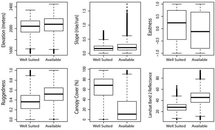
Figure 2. Characterization of habitat classified as well suited as compared to all habitat for all forest types constrained by minimum convex polygon buffered by 500m around known goshawk nest locations within the Cassia Section, Minidoka Ranger District, Sawtooth National Forest in south-central Idaho USA. Boxplots represent median (line), quartiles (box), 1.5 times inter-quartile range (whiskers), and outliers (points).

Figure 3. Habitat model results for full study area as compared to known goshawk nest locations illustrating quantitative and qualitative breakpoints for habitat suitability classification. Data include the cumulative distribution of model results for all 30-meter pixels within the minimum convex polygon encompassing all know goshawk nest locations, cumulative distribution of model results for each of the 80 known nest locations in the model building data set, the difference between these two distributions, the breakpoint for marginal habitat (chosen quantitatively) and the breakpoint for suitable habitat (chosen qualitatively).
For nests located in lodgepole pine the top model included elevation, slope, eastness, ruggedness, canopy cover and Landsat band 4. The nests of goshawks located in lodgepole pine were more often located at lower elevation, with low slope, with east-facing aspect, low ruggedness, high canopy cover, and forest structure with low reflectance of near-infrared (0.75 - 0.9 µm wavelength) [31].
The aspen model classified 83.0% of the total available habitat as poorly suited, 10.5% as marginally suited, and 6.5% as well suited. The lodgepole pine model classified 95.9% of the total habitat as poorly suited, 0.6% of habitat as marginally suited, and 3.5% as well suited.
In validating the models with the reserved set of tests, 83.3% of 12 aspen nests were located in habitat classified as well suited by the aspen model, 8.3% in habitat classified as marginally suited and 8.3% in habitat classified as poorly suited. For lodgepole pine two of the three validation nests were located in habitat classified as well suited by the lodgepole pine model and one of the three in habitat classified as marginally suited. The union of the aspen and lodgepole pine models classified habitat as well suited covers 8.6% of the minimum convex polygon encompassing the known nest locations. This model covers nearly the same amount of territory as the combined model, yet does not perform as well against the validation nests.
4. DISCUSSION
Habitat suitability models can be an effective way to
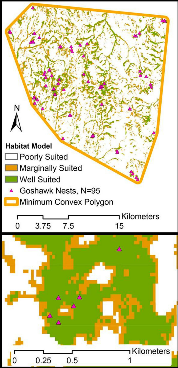
Figure 4. Resulting habitat model for all forest types constrained by minimum convex polygon buffered by 500 meters around known goshawk nest locations within the Cassia Section, Minidoka Ranger District, Sawtooth National Forest in south-central Idaho USA.
quantify the habitat requirements of a species. The habitat variables represented in our model are fairly consistent with other studies. Many studies, including ours, have found that goshawks prefer dense canopy cover on relatively gentle slopes with east facing aspect [5,14-17]. In similar habitat (high-elevation shrub-steppe with fragmented forest stands), Younk and Bechard [15] characterized nest trees with slope aspects north or east facing and a close proximity to water. Distance to water was dropped via model selection from all models that we considered, possibly due to the fairly ubiquitous access to small streams within our study area. The emphasis of lower elevation in our model was no surprise as the higher elevations of our study area have increasing concentration of sub-alpine fir, a species largely insufficient as a structure for the nests of goshawks.
With this application, we have successfully paired down the available habitat in the study area to those areas with a higher likelihood of hosting nests of breeding goshawks. Over 90% of the study area has been eliminated from consideration if we chose to search only the well suited areas. The approach we used in our study classified more area as poor habitat (86.1%), yet performed better on validation (93.3% of reserved nests located in habitat classified as marginal or suitable) as compared with Reich et al. [5] and Mathieu et al. [6]. The success of our model may be the result of a more highly fragmented landscape of our study area as compared to other studies.
The direct use of Landsat imagery in the model selection is a unique approach for our study. Others have introduced an intermediate step of first translating Landsat data into vegetation classes which are then used in model selection [6]. The vegetation class approach is preferred when the goal is to quantify the habitat into easily interpretable forms. However, the lost resolution resulting from the dual processing step, and the general poor performance of classification analysis in mixed sagebrush-aspen habitats, decrease the value of this approach in our area [40].
Our model has substantiated what features may limit nesting by goshawks within the unique environment in southern Idaho. However, it should be noted that this predictive model should be used with care beyond the immediate area. The model is based on the range of values within the study area as sampled with the set of random points. Evaluation of habitats with characteristics beyond the range of values used in our model will likely result in distortion of the predictions [11].
In conclusion, we have generated a strong predictive model for the habitat suitable for hosting breeding goshawks that has performed well against our validation data and compares well with other studies and approaches. This work will assist future surveyors of goshawks in our area and in adjacent areas within the northern Great Basin with similar characteristics.
5. ACKNOWLEDGEMENTS
We thank the U.S.D.A. Forest Service Minidoka Ranger District for their financial, consulting, and equipment support for the completion of this project, particularly wildlife biologist Dena Santini. We also thank Natural Research Ltd. for awarding us the 2011 Mike Madder’s Field Research Award and the Butler family for awarding us the 2012 Michael W. Butler Ecological Research Award.
We received logistic and equipment support from Boise State University’s Raptor Research Center, Idaho Bird Observatory, the Department of Biological Sciences, Inovus Solar, David L. Anderson, and Doug Guillory. We received general consulting from Dr. Jennifer Forbey, from previous goshawk researchers Kristin Hasselblad, Greg Kaltenecker and Susan Patla, and from Boise State University statistician Laura Bond. Thank you to Skye Cooley and David L. Anderson for reviewing this manuscript.
Much of this work was completed using volunteer time from field volunteers including: Jeri Albro, David L. Anderson, Alexis Billings, Karyn deKramer, Michelle Jeffries, Ayla Kaltenecker, Cathy Lapinel, Lauren Lapinel, Kraig Laskowski, Michelle Laskowski, Dusty Perkins, Thurman Pratt, Kerry Rogers, Nicole Rogers, Uri Rogers, Emmy Tyrrell, Cristen Walker, Heidi Ware, Carol Wike, Dave Wike, and Mike Zinn. We would like to thank them all for their hard work and dedication.
![]()
![]()
REFERENCES
- Newton, I. (1979) Population ecology of raptors. Buteo Books, Vermillion.
- Graves, G.R. and Rahbek, C. (2005) Source pool geometry and the assembly of continental avifaunas. Proceedings of the National Academy of Sciences, 102, 7871- 7876. doi:10.1073/pnas.0500424102
- Gotelli, N.J. and Ellison, A.M. (2006) Food-web models predict species abundances in response to habitat change. PLoS Biology, 4, e324. doi:10.1371/journal.pbio.0040324
- Sappington, J.M., Longshore, K.M. and Thompson, D.B. (2007) Quantifying landscape ruggedness for animal habitat analysis: a case study using bighorn sheep in the Mojave Desert. The Journal of Wildlife Management, 71, 1419-1426. doi:10.2193/2005-723
- Reich, R.M., Joy, S.M. and Reynolds, R.T. (2004) Predicting the location of Northern Goshawk nests: modeling the spatial dependency between nest locations and forest structure. Ecological Modelling, 176, 109-133. doi:10.1016/j.ecolmodel.2003.09.039
- Mathieu, R., Seddon, P. and Leiendecker, J. (2006) Predicting the distribution of raptors using remote sensing techniques and geographic information systems: A case study with the Eastern New Zealand Falcon (Falconovaeseelandiae). New Zealand Journal of Zoology, 33, 73- 84. doi:10.1080/03014223.2006.9518432
- Guisan, A. and Zimmermann, N.E. (2000) Predictive habitat distribution models in ecology. Ecological Modelling, 135, 147-186. doi:10.1016/S0304-3800(00)00354-9
- Titus, K. and Mosher, J.A. (1981) Nest-site habitat selected by woodland hawks in the Central Appalachians. The Auk, 98, 270-281.
- Hurlbert, A.H. and Jetz, W. (2007) Species richness, hotspots, and the scale dependence of range maps in ecology and conservation. Proceedings of the National Academy of Sciences, 104, 13384-13389. doi:10.1073/pnas.0704469104
- Wiens, J.A., Rotenberry, J.T. and Horne, B.V. (1987) Habitat occupancy patterns of North American shrubsteppe birds: The effects of spatial scale. Oikos, 48, 132- 147. doi:10.2307/3565849
- O’Reilly, F.J. (1975) On a criterion for extrapolation in normal regression. The Annals of Statistics, 3, 219-222. doi:10.1214/aos/1176343010
- Fielding, A.H. and Haworth, P.F. (1995) Testing the generality of bird-habitat models. Conservation Biology, 9, 1466-1481. doi:10.1046/j.1523-1739.1995.09061466.x
- Squires, J.R. and Reynolds, R.T. (1997) Northern Goshawk (Accipiter gentilis). In: Poole, A., Ed., The Birds of North America Online, Cornell Lab of Ornithology, Ithaca.
- Reynolds, R.T., Meslow, E.C. and Wight, H.M. (1982) Nesting habitat of coexisting accipiter in Oregon. The Journal of Wildlife Management, 46, 124-138. doi:10.2307/3808415
- Younk, J.V. and Bechard, M.J. (1994) Breeding ecology of the Northern Goshawk in high-elevation aspen forests of northern Nevada. In: Block, W.M., Morrison, M.L., and Reiser, M.H., Eds., The Northern Goshawk: Ecology and Management, Proceedings of a Symposium of the Cooper Ornithological Society, Sacramento, 14-15 April 1993, 119-121.
- Finn, S.P., Marzluff, J.M. and Varland, D.E. (2002) Effects of landscape and local habitat attributes on Northern Goshawk site occupancy in western Washington. Forest Science, 48, 427-436.
- La Sorte, F.A., Mannan, R.W., Reynolds, R.T. and Grubb, T.G. (2004) Habitat associations of sympatric Red-Tailed Hawks and Northern Goshawks on the Kaibab Plateau. The Journal of Wildlife Management, 68, 307-317. doi:10.2193/0022-541X(2004)068[0307:HAOSRH]2.0.CO;2
- Krüger, O. (2002) Analysis of nest occupancy and nest reproduction in two sympatric raptors: Common Buzzard Buteo buteo and Goshawk Accipiter gentilis. Ecography, 25, 523-532. doi:10.1034/j.1600-0587.2002.250502.x
- Lõhmus, A. (2005) Are timber harvesting and conservation of nest sites of forest-dwelling raptors always mutually exclusive? Animal Conservation, 8, 443-450. doi:10.1017/S1367943005002349
- Woodbridge, B. and Hargis, C.D. (2006) Northern Goshawk inventory and monitoring technical guide. USDA Forest Service, Washington DC.
- U.S. Forest Service (2003) Sawtooth National Forest revised land and resource management plan. Sawtooth National Forest, Twin Falls.
- U.S. Forest Service (1980) Cassia timber environmental assessment. Sawtooth National Forest, Twin Falls.
- Miller, R.A., Carlisle, J.D. and Bechard, M.J. (In review) Indirect effects of prey abundance on breeding season diet of northern goshawks (accipiter gentilis) within a unique prey landscape. Journal of Raptor Research.
- Kennedy, P.L. and Stahlecker, D.W. (1993) Responsiveness of nesting Northern Goshawks to taped broadcasts of 3 conspecific calls. The Journal of Wildlife Management, 57, 249-257. doi:10.2307/3809421
- Hasselblad, K., Bechard, M. and Bednarz, J.C. (2007) Male Northern Goshawk home ranges in the Great Basin of south-central Idaho. Journal of Raptor Research, 41, 150-155. doi:10.3356/0892-1016(2007)41[150:MNGHRI]2.0.CO;2
- U.S. Geological Survey (1999) National elevation dataset of southcentral Idaho. U.S. Geological Survey, Sioux Falls.
- Roberts, D.W. (1986) Ordination on the basis of fuzzy set theory. Vegetatio, 66, 123-131. doi:10.1007/BF00039905
- Jenness, J.S. (2004) Calculating landscape surface area from digital elevation models. Wildlife Society Bulletin, 32, 829-839. doi:10.2193/0091-7648(2004)032[0829:CLSAFD]2.0.CO;2
- U.S. Geological Survey (2001) National land cover database tree canopy layer. U.S. Geological Survey, Sioux Falls.
- Idaho Department of Environmental Quality (2006) Streams of Idaho (2002 305(b) & 303(d) integrated report—water quality). Idaho Department of Environmental Quality, Boise.
- U.S. Geological Survey (2010) Global land survey (GLS) datasets: 2010. U.S. Geological Survey, Sioux Falls.
- Hijmans, R.J. and Van Etten, J. (2012) Geographic analysis and modeling with raster data. http://raster.r-forge.r-project.org/
- Chambers, J.M. and Hastie, T. (1992) Statistical models in S. Wadsworth & Brooks/Cole Advanced Books & Software, Pacific Grove.
- Cliff, A.D. and Ord, J.K. (1981) Spatial processes : Models & applications. Pion, London.
- Ottaviani, D., Lasinio, G.J. and Boitani, L. (2004) Two statistical methods to validate habitat suitability models using presence-only data. Ecological Modelling, 179, 417-443. doi:10.1016/j.ecolmodel.2004.05.016
- R Development Core Team (2012) R: A language and environment for statistical computing. http://www.R-project.org
- VanDerWal, J., Falconi, L., Januchowski, S., Shoo, L. and Storlie, C. (2012) Species distribution modelling tools. http://www.rforge.net/SDMTools/
- Bivand, R. (2012) Spatial dependence: Weighting schemes, statistics and models. http://cran.r-project.org/web/packages/spdep/index.html
- ESRI (2012) ArcMap 10.1. http://www.esri.com/
- Lowry, J., et al. (2007) Mapping moderate-scale landcovers over very large geographic areas within a collaborative framework: A case study of the southwest regional gap analysis project (SWReGAP). Remote Sensing of Environment, 108, 59-73. doi:10.1016/j.rse.2006.11.008.